Correção IME 2027 · Português e InglêsAcompanhe a resolução de cada questão da 2ª fase, ao vivoAcompanhar
IA ao vivo / ITA 2027 · 2ª fase · Física

COMPARE OS RACIOCÍNIOS

Questão 1 (Física)

Questão discursiva: a banca não divulga gabarito oficial. 2 (Física) →

A questão

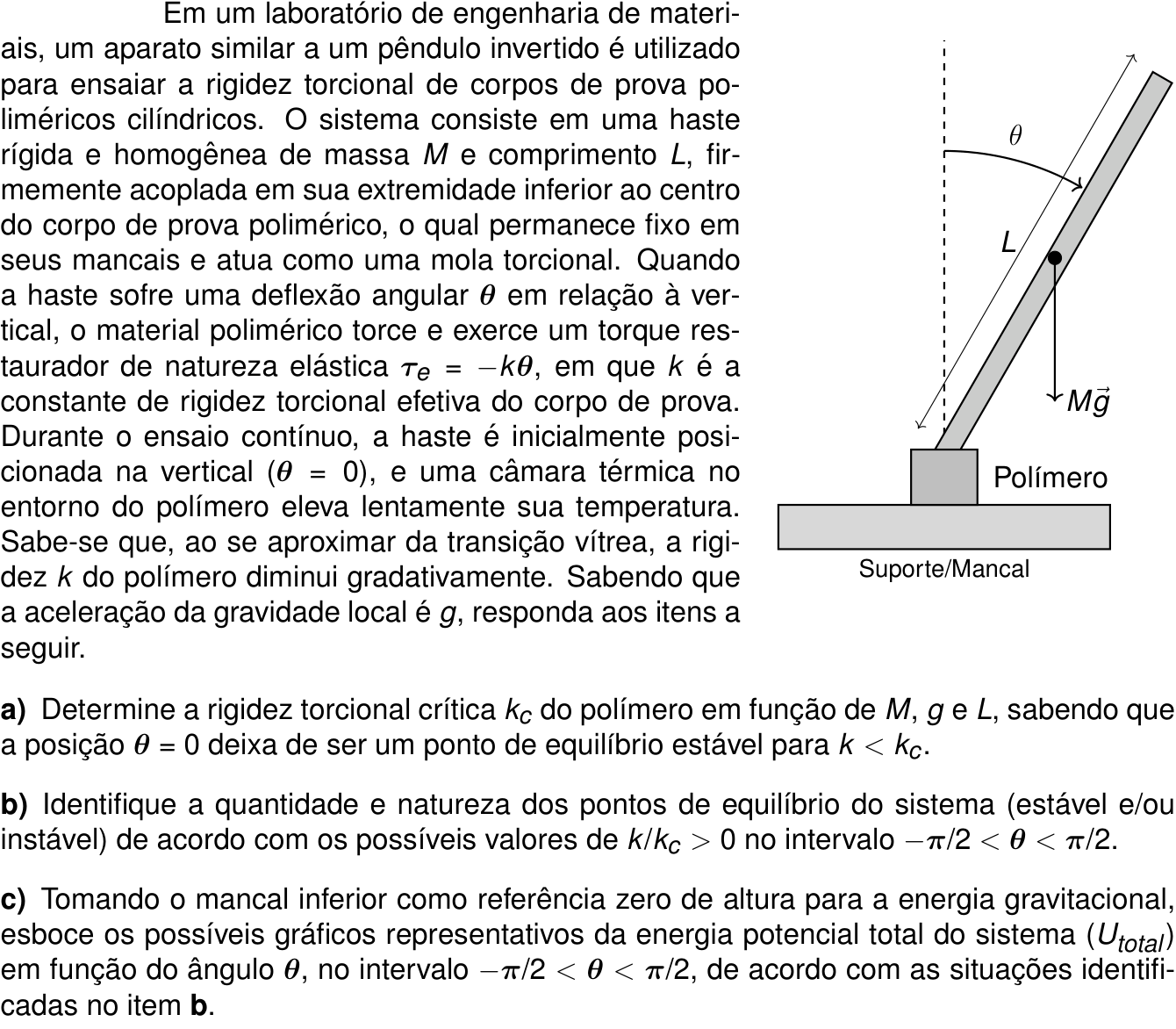
Texto de apoio da questão 1 (Física) Questão 1 (Física)

Resposta de referência

a) k_c=MgL/2. b) Definindo r=k/k_c>0: para r\ge1, há apenas \theta=0, estável; para 2/\pi<r<1, há três equilíbrios: 0, instável, e \pm\theta_0, estáveis, com \sin\theta_0/\theta_0=r; para 0<r\le2/\pi, há apenas 0, instável. c) U(\theta)=k\theta^2/2+(MgL/2)\cos\theta, função par com U(0)=MgL/2. Os perfis são: mínimo único em 0 para r\ge1 (quártico na origem quando r=1); poço duplo, com máximo central e dois mínimos simétricos, para 2/\pi<r<1; máximo central e decrescimento com |\theta|, sem mínimos no intervalo, para 0<r\le2/\pi.

Segundo a resolução dos cursinhos Farias Brito e Poliedro. A banca não publica gabarito das questões discursivas.

Respostas das IAs

GPT-6 Astra

Respondeu · bate com a resposta de referência dos cursinhos

a) k_c=MgL/2; b) para r=k/k_c\ge1, 1 equilíbrio estável; para 2/\pi<r<1, 2 estáveis e 1 instável; para 0<r\le2/\pi, 1 instável; c) U_{\text{total}}=\frac{k\theta^2}{2}+\frac{MgL}{2}\cos\theta, com os perfis esboçados acima.

levou 1 min 20 s

Como pensou

a) Rigidez torsional crítica

O peso atua no centro de massa da haste, a uma distância L/2 da articulação. Tomando como positivo o sentido de aumento de \theta, o torque resultante é

\tau(\theta)=\frac{MgL}{2}\sin\theta-k\theta.

Para pequenas deflexões,

\tau(\theta)\approx \left(\frac{MgL}{2}-k\right)\theta.

O equilíbrio vertical é estável quando esse torque se opõe à deflexão, isto é, quando k>MgL/2. Portanto,

\boxed{k_c=\frac{MgL}{2}}.

b) Quantidade e natureza dos equilíbrios

Definindo r=k/k_c>0, a condição de equilíbrio é

\sin\theta=r\theta.

Assim, \theta=0 é sempre um equilíbrio. Para os equilíbrios não nulos,

r=\frac{\sin\theta}{\theta}.

A função \sin\theta/\theta é par e, para 0<\theta<\pi/2, decresce estritamente de 1 até 2/\pi, sem atingir esses valores. Logo, existem dois equilíbrios não nulos, \pm\theta_e, somente quando

\frac2\pi<r<1, \qquad \frac{\sin\theta_e}{\theta_e}=r.

Para verificar sua estabilidade, calculamos

\tau'(\theta_e) =k_c\left(\cos\theta_e-\frac{\sin\theta_e}{\theta_e}\right)<0,

pois \sin\theta_e>\theta_e\cos\theta_e para 0<\theta_e<\pi/2. Portanto, ambos são estáveis.

Na origem, \tau'(0)=k_c(1-r): ela é estável para r>1 e instável para r<1. No caso crítico r=1,

\tau=k_c(\sin\theta-\theta),

que tem sinal oposto ao de \theta. Logo, a origem continua estável, embora o termo linear do torque seja nulo.

A classificação completa é:

Valor de r=k/k_c Equilíbrios em (-\pi/2,\pi/2) Natureza
r>1 Apenas \theta=0 Estável
r=1 Apenas \theta=0 Estável, com restauração não linear
2/\pi<r<1 0,\,-\theta_e,\,+\theta_e Origem instável; outros dois estáveis
0<r\le2/\pi Apenas \theta=0 Instável

Em r=2/\pi, os equilíbrios não nulos estariam em \theta=\pm\pi/2, excluídos do intervalo.

c) Energia potencial e esboços

A altura do centro de massa é

h=\frac L2\cos\theta.

Adotando energia elástica nula na configuração sem torção,

\boxed{U_{\text{total}}(\theta) =\frac{k\theta^2}{2}+\frac{MgL}{2}\cos\theta}.

Equivalentemente,

\frac{U_{\text{total}}}{k_c} =\frac r2\theta^2+\cos\theta.

Todos os gráficos são pares e passam por U(0)=k_c. Além disso,

U'(\theta)=k_c(r\theta-\sin\theta), \qquad U''(\theta)=k_c(r-\cos\theta).

Os perfis qualitativos são os seguintes, com extremidades excluídas e alturas não em escala:

       r > 1                       r = 1
 U                           U
 ↑   \         /             ↑   \           /
 |    \       /              |    \         /
 |     \     /               |     \_______/
 |      \___/                |
 +--------0--------→ θ       +---------0--------→ θ


     2/π < r < 1                 0 < r ≤ 2/π
 U                           U
 ↑  \             /          ↑        ___
 |   \    /\     /           |      /     \
 |    \__/  \___/            |    /         \
 |                           |   /           \
 +---------0-------→ θ       +---------0--------→ θ
  • r>1: curva estritamente convexa, com mínimo em \theta=0.
  • r=1: mínimo mais achatado na origem. De fato,
U(\theta)=k_c+\frac{k_c}{24}\theta^4+O(\theta^6).
  • 2/\pi<r<1: perfil de poço duplo, com máximo local em 0 e mínimos em \pm\theta_e.
  • 0<r\le2/\pi: máximo em 0, com a energia diminuindo à medida que |\theta| aumenta, sem mínimos no intervalo. Para r=2/\pi, a inclinação tende a zero nas extremidades.

Para fixar também as alturas das bordas,

\lim_{\theta\to\pm\pi/2}U(\theta)=\frac{k\pi^2}{8}.

Assim, no perfil de poço duplo, essas alturas podem ficar abaixo, iguais ou acima de U(0), conforme r seja menor, igual ou maior que 8/\pi^2.

Resposta final: a) k_c=MgL/2; b) para r=k/k_c\ge1, 1 equilíbrio estável; para 2/\pi<r<1, 2 estáveis e 1 instável; para 0<r\le2/\pi, 1 instável; c) U_{\text{total}}=\frac{k\theta^2}{2}+\frac{MgL}{2}\cos\theta, com os perfis esboçados acima.

GPT-6.1 Sol

Respondeu · bate com a resposta de referência dos cursinhos

a) k_c=MgL/2; b) k/k_c\ge1: um equilíbrio estável; 2/\pi<k/k_c<1: três, sendo 0 instável e \pm\theta_e estáveis, com \sen\theta_e/\theta_e=k/k_c; 0<k/k_c\le2/\pi: um equilíbrio instável; c) U=\frac12k\theta^2+\frac{MgL}{2}\cos\theta, com os perfis esboçados acima.

levou 1 min 02 s

Como pensou
**Considering W shapes** I need to mention that W shapes may have endpoints below the central point. So, a table might allow for a derivative pattern here. I could sketch the W with side arms, but I’d leave the vertical truncation unspecified. It’s important to note that the height can vary and isn't always exact. That should give a clearer understanding of the concept!

O centro de massa da haste está à distância L/2 do eixo de rotação. Tomando como positivo o sentido de aumento de \theta, o torque resultante é

\tau(\theta)=\frac{MgL}{2}\sen\theta-k\theta.

a) Rigidez crítica

Para pequenas deflexões,

\tau(\theta)\simeq \left(\frac{MgL}{2}-k\right)\theta.

O equilíbrio vertical é estável quando esse torque se opõe à deflexão, isto é, quando k>MgL/2. Portanto,

\boxed{k_c=\frac{MgL}{2}}.

b) Quantidade e natureza dos equilíbrios

Definindo r=k/k_c>0, a condição de equilíbrio é

\sen\theta=r\theta.

Assim, \theta=0 é sempre um equilíbrio. Para os equilíbrios não nulos,

r=\frac{\sen\theta}{\theta}.

No intervalo 0<\theta<\pi/2, a função \sen\theta/\theta é estritamente decrescente, pois

\frac{d}{d\theta}\left(\frac{\sen\theta}{\theta}\right) =\frac{\theta\cos\theta-\sen\theta}{\theta^2}<0,

e seus limites são

\lim_{\theta\to0}\frac{\sen\theta}{\theta}=1, \qquad \lim_{\theta\to\pi/2}\frac{\sen\theta}{\theta}=\frac2\pi.

Logo, existem dois equilíbrios não nulos, simétricos, somente se

\frac2\pi<r<1.

Para analisar a estabilidade, usamos

U''(\theta)=k-k_c\cos\theta.

Na origem,

U''(0)=k_c(r-1),

de modo que ela é estável para r>1 e instável para r<1.

Nos equilíbrios não nulos \pm\theta_e,

U''(\pm\theta_e) =k_c\left(\frac{\sen\theta_e}{\theta_e}-\cos\theta_e\right)>0.

Portanto, ambos são estáveis.

No caso crítico r=1, é necessário ir além da aproximação quadrática:

U(\theta)=k_c+\frac{k_c}{24}\theta^4+O(\theta^6).

Assim, a origem continua sendo um mínimo estável, embora não haja termo restaurador linear.

Em resumo:

Valor de r=k/k_c Equilíbrios em (-\pi/2,\pi/2)
r>1 Um: \theta=0, estável
r=1 Um: \theta=0, estável, com mínimo quártico
2/\pi<r<1 Três: 0, instável; \pm\theta_e, estáveis
0<r\le 2/\pi Um: \theta=0, instável

Em r=2/\pi, as soluções adicionais seriam \theta=\pm\pi/2, mas esses pontos não pertencem ao intervalo dado.

c) Energia potencial e esboços

Como a altura do centro de massa é h=(L/2)\cos\theta,

\boxed{U(\theta)=\frac12k\theta^2+\frac{MgL}{2}\cos\theta}

ou

\boxed{\frac{U(\theta)}{k_c}=\frac r2\theta^2+\cos\theta}.

Todos os gráficos são simétricos em relação ao eixo vertical e passam por

U(0)=k_c.

Nas extremidades abertas do intervalo,

\lim_{\theta\to\pm\pi/2}U(\theta)=\frac{k\pi^2}{8}.

Os esboços qualitativos são:

• r>1: um único mínimo, com concavidade para cima em todo o intervalo.

 U
 │ \           /
 │  \         /
 │   \_______/
 └────────────── θ
         0

Próximo da origem, U-U(0)\simeq \tfrac12(k-k_c)\theta^2.

• r=1: um único mínimo, mais achatado na origem.

 U
 │ \             /
 │  \           /
 │   \_________/
 └──────────────── θ
          0

Nesse caso, U-U(0)\simeq k_c\theta^4/24.

• 2/\pi<r<1: dois mínimos simétricos e um máximo central.

 U
 │ \                 /
 │  \       /\      /
 │   \_____/  \____/
 └──────────────────── θ
       -θe   0   θe

As alturas das extremidades em relação ao máximo central dependem de r, conforme U(\pm\pi/2)\to k\pi^2/8.

• 0<r\le2/\pi: um único máximo central; a energia cresce até \theta=0 e depois decresce.

 U
 │       _____
 │     /       \
 │ ___/         \___
 └──────────────────── θ
           0

Para r=2/\pi, a inclinação tende a zero nas duas extremidades; para r<2/\pi, não.

Resposta final: a) k_c=MgL/2; b) k/k_c\ge1: um equilíbrio estável; 2/\pi<k/k_c<1: três, sendo 0 instável e \pm\theta_e estáveis, com \sen\theta_e/\theta_e=k/k_c; 0<k/k_c\le2/\pi: um equilíbrio instável; c) U=\frac12k\theta^2+\frac{MgL}{2}\cos\theta, com os perfis esboçados acima.

GPT-6 Luna

Respondeu · bate com a resposta de referência dos cursinhos

a) k_c=MgL/2; b) 0<k/k_c\le2/\pi: só \theta=0, instável; 2/\pi<k/k_c<1: \theta=0 instável e \pm\theta_* estáveis; k/k_c=1: \theta=0 estável degenerado; k/k_c>1: \theta=0 estável; c) gráficos com os extremos e formatos descritos acima.

levou 48 s

Como pensou
**Evaluating graph shape** I’m considering that when r equals 1, the shape of the graph appears distinct and flatter compared to values greater than 1. It might be worth mentioning the critical quartic here. For r values less than 2/pi, I'm thinking that the curve could potentially dip down towards the edges. Got to keep that in mind as I explore these graph behaviors!**Analyzing positive U values** I’m thinking about very small positive U values, notably boundary values, with no extra extremes. I need to sketch possible graphs that represent different situations with bifurcations at specific r values: 0<r≤2/π; 2/π<r<1; r=1; r>1. At r=2/π, the derivative vanishes, resulting in a boundary horizontal graph. I’m also considering gravitational torque on an inverted rod with a pivot and positive theta; the equations need careful analysis, particularly using small-angle approximation. This is good!**Considering theta and bifurcation** I’m thinking about small theta values where sin θ is approximately equal to theta, particularly in relation to bifurcation. The interval is ±π/2, and I need to consider all equilibria based on the ratio k/kc. The prompt suggests using the small angle approximation, especially when theta is much less than 1. For this problem, it seems important to look at the existence thresholds involving exact sine, particularly at boundary values like 2/π, to count equilibria accurately and understand stability.**Examining sine and stability** I think I shouldn’t approximate sine unless I’m expanding near zero. I’m curious about the classification of stable vs. unstable points at intermediate values and specifically at k=kc using exact conditions. It's crucial that I confirm equilibrium at θ=0 when k equals kc. I can use Lyapunov’s stability method with quartic equations. The net torque calculation involves gravitational and spring forces, represented by the equation τ_net = A sin θ - kθ. This is shaping up to be an interesting analysis!**Analyzing boundary values** I'm considering how the curve rises at the boundaries and whether the boundary values might be lower than the central value. The endpoint potential is something like rπ²/8, and I compare different values. If r is greater than 2/π, the endpoint value exceeds π/4, but could it be lower than the central value if r is below a certain threshold? I need to note that local minima can occur, but the potential global minimum might be at an open endpoint, depending on the values of r.**Evaluating curve behavior** I'm exploring how the endpoint value compares to the center, realizing that it's not always relevant for the plot. The central point is a local maximum, and it's possible for the endpoint to be below the center, resulting in a curve that drops and then rises. For r equal to 1 and above, the function shows monotonic increase from zero to the boundary. When r is greater than 1, the curvature seems convex, and the second derivative is positive across the domain.**Analyzing equations and approximations** The user asked me to solve a problem, and I’m considering the initial information, like when sin≈theta applies. They might expect us to use a small angle approximation to find thresholds. However, if we assume sinθ≈θ for all angles, the equilibrium equation leads to k=kc for any theta, which seems odd. It could be that they're looking for critical and local analysis instead. I wonder if they expect cubic sine expansion or Taylor expansion details, which aren't provided. The wording suggests a specific instruction, indicating perhaps not to use cubic terms. To determine stability, I'd need to ensure sinθ<θ without approximation.**Exploring approximations in equations** I'm considering how I can invoke sinθ<θ for positive θ, which is a known relationship. I think energy might be better expanded using cos, but if I'm only given that sin≈theta, it seems like the higher order terms get lost at critical torque differentials. This could lead to identifying the situation as marginal or neutral. However, I suspect that the physically nonlinear approach gives more stability overall. It’s interesting how these details play into the analysis!**Considering graph representation** I think it's important to present a robust solution that might include a verbal sketch with key points and trends. User wants an exam answer showing development, so I should definitely consider that. I can draw a simple ASCII conceptual graph with axes, but I need to be mindful of not cluttering it with multiple regimes and symmetry. Balancing clarity and detail is essential here!**Evaluating potential energy of a spring** I'm considering the potential energy of a torsional spring at specific angles. At θ=0, I determine that the mechanical torque due to gravity is consistent with the equations I'm referencing. I find interesting relationships between potential energy and angle values, noting that the graph's endpoints rise from minima, remaining symmetric. For r=1, I notice a flat region near the origin, and as r increases, the shape resembles a bowl. Finally, I plan to present my findings in Portuguese.

Seja A=\dfrac{MgL}{2}. O centro de massa da haste está a uma altura z=\dfrac L2\cos\theta em relação ao mancal inferior. Assim, a energia potencial total, a menos de uma constante, é

U(\theta)=A\cos\theta+\frac12 k\theta^2.

O torque resultante é

\tau=-\frac{dU}{d\theta}=A\sin\theta-k\theta.

a) Rigidez torsional crítica

Para pequenos ângulos,

\tau\simeq (A-k)\theta.

A posição vertical é estável quando o torque resultante é restaurador, isto é, quando k>A. Portanto, a rigidez crítica é

\boxed{k_c=A=\frac{MgL}{2}}.

b) Pontos de equilíbrio e sua natureza

Definindo r=k/k_c, a condição de equilíbrio é

r\theta=\sin\theta.

Além de \theta=0, possíveis equilíbrios não nulos satisfazem

r=\frac{\sin\theta}{\theta}.

No intervalo considerado, \sin\theta/\theta diminui de 1 até 2/\pi quando \theta vai de 0 a \pi/2. Logo:

  • 0<r\le 2/\pi: há apenas \theta=0, que é instável. Para r=2/\pi, as soluções não nulas estariam em \theta=\pm\pi/2, fora do intervalo.
  • 2/\pi<r<1: há três equilíbrios: \theta=0, instável, e \theta=\pm\theta_*, estáveis, em que \sin\theta_*/\theta_*=r.
  • r=1: há apenas \theta=0. É um mínimo estável degenerado, pois
U(\theta)=k_c\left(1+\frac{\theta^4}{24}+\cdots\right)

perto de \theta=0.

  • r>1: há apenas \theta=0, que é estável.

Nos equilíbrios não nulos, a estabilidade também decorre de

U''(\theta_*)=k_c\left(\frac{\sin\theta_*}{\theta_*}-\cos\theta_*\right)>0.

c) Gráficos de U_{\text{total}}

Em unidades de k_c, a energia pode ser representada por

\frac{U(\theta)}{k_c}=\cos\theta+\frac r2\theta^2.

Ela é simétrica em relação a \theta=0. Os esboços devem ter as seguintes características:

  • 0<r\le 2/\pi: máximo em \theta=0; a energia decresce em direção às duas extremidades. Para r=2/\pi, a inclinação tende a zero nas extremidades.
  • 2/\pi<r<1: máximo em \theta=0 e mínimos em \theta=\pm\theta_*.
  • r=1: mínimo plano em \theta=0, com variação proporcional a \theta^4 perto da origem.
  • r>1: mínimo em \theta=0, com curvatura positiva.

Resposta final: a) k_c=MgL/2; b) 0<k/k_c\le2/\pi: só \theta=0, instável; 2/\pi<k/k_c<1: \theta=0 instável e \pm\theta_* estáveis; k/k_c=1: \theta=0 estável degenerado; k/k_c>1: \theta=0 estável; c) gráficos com os extremos e formatos descritos acima.

Claude Fable 5.1

Respondeu · bate com a resposta de referência dos cursinhos

a) k_c = MgL/2; b) k/k_c \ge 1: só θ = 0, estável (marginal em k=k_c); 2/\pi<k/k_c<1: θ = 0 instável e θ = ±θ₀ (sen θ₀/θ₀ = k/k_c) estáveis; k/k_c\le 2/\pi: só θ = 0, instável; c) U=\tfrac12 k\theta^2+\tfrac{MgL}{2}\cos\theta: "U" com mínimo em 0 (k>k_c), fundo achatado (k=k_c), poço duplo "W" com máximo em 0 e mínimos em ±θ₀ (2/\pi<k/k_c<1), "∩" com máximo em 0 (k/k_c\le 2/\pi).

levou 33 s

Como pensou
I'm setting up the inverted pendulum problem with a torsional spring at the pivot, writing the potential energy as the spring term plus gravitational contribution, then finding equilibrium by setting its derivative to zero, giving kθ = Mg(L/2)sinθ. Checking stability at θ=0, I find the critical spring constant k_c = MgL/2, above which the upright position is stable. Rewriting the equilibrium condition as sinθ/θ = k/k_c, I analyze how many solutions exist depending on the ratio k/k_c: for k/k_c ≥ 1, only θ=0 exists and is stable (with a quartic correction at exactly k=k_c); for 2/π < k/k_c < 1, three equilibria appear with θ=0 unstable and the two nonzero solutions stable; and for k/k_c ≤ 2/π, θ=0 remains the sole but unstable equilibrium. I verify the stability of the nonzero equilibria by checking that tanθ₀ > θ₀, confirming they're stable, and note the problem's hint to use small-angle approximations where appropriate even though a full treatment requires the 2/π threshold. Now I'm sketching the shape of U(θ) in words across regimes: for k above k_c it's a single convex well centered at zero; at k_c it flattens into a quartic minimum; between 2/π·k_c and k_c it becomes a double well with a local max at zero and minima at ±θ₀; and below 2/π·k_c the origin becomes a maximum with U decreasing monotonically out to ±π/2, where U = kπ²/8.

Montagem do problema

Tomando o mancal (pivô) como origem, o centro de massa da haste está à altura (L/2)cosθ. A energia potencial total (gravitacional + elástica da mola torcional) é

U(\theta)=\frac{1}{2}k\theta^{2}+\frac{MgL}{2}\cos\theta .

Condição de equilíbrio: \dfrac{dU}{d\theta}=k\theta-\dfrac{MgL}{2}\sin\theta=0.

Estabilidade: \dfrac{d^2U}{d\theta^2}=k-\dfrac{MgL}{2}\cos\theta (estável se > 0).

a) Em θ = 0: U''(0)=k-\dfrac{MgL}{2}. A posição vertical é estável enquanto k>\dfrac{MgL}{2} e deixa de sê‑lo para k<\dfrac{MgL}{2}. Logo

k_c=\frac{MgL}{2}.

(Com sen θ ≈ θ: torque líquido -(k-k_c)\theta; é restaurador só se k>k_c.)

b) A equação de equilíbrio pode ser escrita como

\frac{\sin\theta}{\theta}=\frac{k}{k_c}.

θ = 0 é sempre equilíbrio. No intervalo -\pi/2<\theta<\pi/2, a função sen θ/θ é par, vale 1 em θ = 0 e decresce monotonicamente até 2/\pi em |\theta|\to\pi/2. Então:

  • k/k_c > 1: um único equilíbrio, θ = 0, estável (U''(0)=k-k_c>0).
  • k/k_c = 1: um único equilíbrio, θ = 0, ainda estável, mas marginal (não harmônico): U\approx \text{const}+k_c\theta^4/24.
  • 2/π < k/k_c < 1: três equilíbrios: θ = 0 instável (U''(0)<0) e dois pontos simétricos θ = ±θ₀, com \sin\theta_0/\theta_0=k/k_c, estáveis (pois U''(\pm\theta_0)=k_c(\sin\theta_0/\theta_0-\cos\theta_0)>0, já que tan θ₀ > θ₀).
  • 0 < k/k_c ≤ 2/π: um único equilíbrio no intervalo, θ = 0, instável (os mínimos ±θ₀ caem fora de |θ| < π/2; a haste tomba até o limite do intervalo).

c) Gráficos de U(\theta)=\tfrac12 k\theta^2+k_c\cos\theta, todos pares, com U(0)=k_c=MgL/2 e U(\pm\pi/2)=k\pi^2/8:

  1. k > k_c: curva em forma de "U" (côncava para cima), com um único mínimo em θ = 0 (poço parabólico, oscilação harmônica em torno da vertical).
  2. k = k_c: curva com fundo achatado em θ = 0 (mínimo quártico), subindo para os dois lados.
  3. 2/π < k/k_c < 1: "poço duplo" (forma de W): máximo local em θ = 0 e dois mínimos simétricos em ±θ₀, com U voltando a crescer até ±π/2.
  4. k/k_c ≤ 2/π: curva em forma de "∩" no intervalo: máximo em θ = 0 e decrescendo monotonicamente até as bordas ±π/2 (os mínimos ficam fora do intervalo).

Resposta final: a) k_c = MgL/2; b) k/k_c \ge 1: só θ = 0, estável (marginal em k=k_c); 2/\pi<k/k_c<1: θ = 0 instável e θ = ±θ₀ (sen θ₀/θ₀ = k/k_c) estáveis; k/k_c\le 2/\pi: só θ = 0, instável; c) U=\tfrac12 k\theta^2+\tfrac{MgL}{2}\cos\theta: "U" com mínimo em 0 (k>k_c), fundo achatado (k=k_c), poço duplo "W" com máximo em 0 e mínimos em ±θ₀ (2/\pi<k/k_c<1), "∩" com máximo em 0 (k/k_c\le 2/\pi).

Claude Opus 5.5

Respondeu · bate com a resposta de referência dos cursinhos

a) k_c = MgL/2; b) para k/k_c ≥ 1, um equilíbrio estável (θ = 0); para 2/π < k/k_c < 1, três equilíbrios: θ = 0 instável e ±θ* estáveis, com senθ*/θ* = k/k_c; para k/k_c ≤ 2/π, um equilíbrio instável (θ = 0); c) U = ½kθ² + (MgL/2)cosθ, com gráfico em "U" (mínimo em 0), em "W" (máximo em 0 e mínimos em ±θ*) e em "∩" (máximo em 0, decrescendo até ±π/2), respectivamente.

levou 24 s

Como pensou
I'm analyzing the inverted pendulum with a torsional spring: gravity torque MgL/2 sinθ is destabilizing while the spring torque −kθ restores, so stability requires k exceeding the critical value MgL/2. For nonzero equilibria I'm solving sinθ/θ = k/kc within the range (−π/2, π/2). Since sinθ/θ runs from 1 at θ=0 down to 2/π at the endpoints, I find three regimes: when k/kc ≥ 1 only θ=0 exists and is stable; when 2/π < k/kc < 1 a pitchfork occurs giving an unstable θ=0 with two symmetric stable equilibria ±θ*; and when k/kc ≤ 2/π only θ=0 exists and it's unstable, since the restoring spring torque can't overcome gravity anywhere in the interval. Writing the potential energy as U = kc cosθ + kθ²/2, I'm now sketching the three cases—a single well, a double-well "W" shape, and a single hump—to visualize how the equilibria appear.

Considero θ > 0 para o lado indicado na figura. O peso atua no centro de massa, a L/2 do mancal.

a) Rigidez crítica

O torque resultante em relação ao mancal é

τ(θ) = Mg(L/2) senθ − kθ.

Para θ ≪ 1, com senθ ≈ θ:

τ ≈ (MgL/2 − k)θ.

A posição θ = 0 é estável quando o torque é restaurador, ou seja, quando k > MgL/2. Para k < MgL/2 o torque afasta a haste da vertical e o equilíbrio fica instável. Logo:

k_c = MgL/2

b) Pontos de equilíbrio

O equilíbrio exige τ = 0:

k_c senθ = kθ ⟹ θ = 0 ou senθ/θ = k/k_c.

No intervalo 0 < |θ| < π/2, a função senθ/θ decresce de 1 (quando θ → 0) até 2/π (quando θ → π/2, valor que não é atingido). A estabilidade vem do sinal de dτ/dθ = k_c cosθ − k, que deve ser negativo para equilíbrio estável.

  • k/k_c ≥ 1: existe um único equilíbrio, θ = 0, e ele é estável.

    • Para θ ≠ 0 vale k_c senθ < kθ, então o torque é sempre restaurador.
    • No caso limite k = k_c, a estabilidade vem do termo de ordem superior: k_c(senθ − θ) tem sinal oposto a θ.
  • 2/π < k/k_c < 1: existem três equilíbrios.

    • θ = 0 é instável, pois dτ/dθ = k_c − k > 0.
    • Os pontos simétricos θ = ±θ*, com senθ*/θ* = k/k_c, são estáveis. Neles, dτ/dθ = k_c(cosθ* − senθ*/θ*) < 0, porque tanθ* > θ*.
  • 0 < k/k_c ≤ 2/π: existe um único equilíbrio, θ = 0, e ele é instável.

    • A equação senθ/θ = k/k_c não tem solução em |θ| < π/2.
    • O torque k_c senθ − kθ tem o mesmo sinal de θ, ou seja, empurra a haste para longe da vertical em todo o intervalo.

c) Energia potencial

Tomando o mancal como referência de altura:

U_total(θ) = ½kθ² + Mg(L/2)cosθ = ½kθ² + k_c cosθ.

U_total é par em θ e vale k_c em θ = 0. Os esboços em −π/2 < θ < π/2 são:

  1. k ≥ k_c: curva em forma de "U" (tipo parábola), com um único mínimo em θ = 0, onde U = k_c. A curva cresce até U(±π/2) = kπ²/8.

  2. 2/π < k/k_c < 1: curva em forma de "W", com máximo local em θ = 0 (U = k_c) e dois mínimos simétricos em ±θ*. Nas extremidades U volta a subir até kπ²/8.

  3. k/k_c ≤ 2/π: curva em forma de "∩", com máximo em θ = 0 (U = k_c). A curva decresce monotonicamente para os dois lados até U(±π/2) = kπ²/8, que é menor que k_c.

Resposta final: a) k_c = MgL/2; b) para k/k_c ≥ 1, um equilíbrio estável (θ = 0); para 2/π < k/k_c < 1, três equilíbrios: θ = 0 instável e ±θ* estáveis, com senθ*/θ* = k/k_c; para k/k_c ≤ 2/π, um equilíbrio instável (θ = 0); c) U = ½kθ² + (MgL/2)cosθ, com gráfico em "U" (mínimo em 0), em "W" (máximo em 0 e mínimos em ±θ*) e em "∩" (máximo em 0, decrescendo até ±π/2), respectivamente.

Claude Sonnet 5.5

Respondeu · bate com a resposta de referência dos cursinhos

a) k_c = MgL/2; b) k/k_c ≥ 1: 1 equilíbrio (θ=0, estável); 2/π < k/k_c < 1: 3 equilíbrios (θ=0 instável, ±θ₀ estáveis); k/k_c ≤ 2/π: 1 equilíbrio (θ=0, instável); c) gráficos simétricos: poço único (k ≥ k_c), poço duplo com máximo local em 0 (2/π < k/k_c < 1), máximo único em 0 (k/k_c ≤ 2/π).

levou 19 s

Como pensou
I'm setting up the energy balance for the rod with potential energy from the spring torque and gravity acting on the center of mass. Taking the derivative and checking the second-order condition at θ=0, I find the critical spring constant where stability switches is kc = MgL/2. Now I'm solving the full equilibrium equation kθ = kc sinθ, which reduces to comparing sinθ/θ against the ratio k/kc. I'm working through the three regimes: for k ≥ kc only θ=0 exists and is stable; for 2/π < k/kc < 1 there are three equilibria with θ=0 becoming unstable and the two symmetric nonzero solutions being stable (confirmed via the second derivative test using tanθ>θ); and for k/kc ≤ 2/π only the unstable θ=0 solution remains. I'm now moving to sketch the potential energy curves for each of these cases, starting with the single-well parabola-like shape when k/kc > 1.

Montagem. Com a altura do centro de massa em (L/2)cosθ, a energia potencial total (elástica + gravitacional) é

U(θ) = ½kθ² + Mg(L/2)cosθ.

a) Os equilíbrios satisfazem

dU/dθ = kθ − (MgL/2)senθ = 0.

θ = 0 é sempre solução. Sua estabilidade é dada por

d²U/dθ²|₀ = k − MgL/2.

O equilíbrio é estável se essa grandeza for positiva e deixa de ser estável quando k < MgL/2. Logo

k_c = MgL/2.

Para θ ≪ 1, senθ ≈ θ, e o resultado é coerente: kθ ≈ k_cθ.

b) Escrevendo k_c = MgL/2, os equilíbrios fora da origem satisfazem

kθ = k_c senθ, ou seja, senθ/θ = k/k_c.

No intervalo (−π/2, π/2), a função senθ/θ é par e decresce de 1 (em θ→0) até 2/π (em θ→±π/2, extremos excluídos). Portanto só há soluções θ ≠ 0 se 2/π < k/k_c < 1.

Para a estabilidade de um equilíbrio θ₀ ≠ 0, usa-se k = k_c senθ₀/θ₀:

U'' = k_c(senθ₀/θ₀ − cosθ₀) = k_c cosθ₀(tgθ₀/θ₀ − 1) > 0,

pois tgθ₀ > θ₀. Esses equilíbrios são, portanto, estáveis.

Resumo:

  • k/k_c ≥ 1: um único equilíbrio, θ = 0, estável. Em k = k_c, U'' = 0, mas U ≈ k_cθ⁴/24 + const, então ainda é um mínimo (estável).
  • 2/π < k/k_c < 1: três equilíbrios. θ = 0 é instável e ±θ₀ são estáveis, simétricos, com θ₀ crescendo conforme k/k_c diminui.
  • k/k_c ≤ 2/π: um único equilíbrio, θ = 0, instável. Não há outros no intervalo aberto.

c) Todos os gráficos de U(θ) são pares (simétricos em θ), com U(0) = MgL/2 = k_c.

  1. k > k_c: curva com um único poço, mínimo em θ = 0, parecida com uma parábola que se achata (U'' > 0).
  2. k = k_c: um único mínimo em θ = 0, muito plano, tipo θ⁴.
  3. 2/π < k/k_c < 1: poço duplo. Há um máximo local em θ = 0 e dois mínimos simétricos em ±θ₀, com U(±θ₀) < U(0). Depois dos mínimos, a curva sobe até as bordas ±π/2, onde U = kπ²/8.
  4. k/k_c ≤ 2/π: um único máximo em θ = 0, e U decresce monotonicamente de cada lado até ±π/2, onde U = kπ²/8 < U(0). Não há mínimo no intervalo.

Resposta final: a) k_c = MgL/2; b) k/k_c ≥ 1: 1 equilíbrio (θ=0, estável); 2/π < k/k_c < 1: 3 equilíbrios (θ=0 instável, ±θ₀ estáveis); k/k_c ≤ 2/π: 1 equilíbrio (θ=0, instável); c) gráficos simétricos: poço único (k ≥ k_c), poço duplo com máximo local em 0 (2/π < k/k_c < 1), máximo único em 0 (k/k_c ≤ 2/π).

Grok 4.7

Respondeu · bate com a resposta de referência dos cursinhos

a) \frac12 MgL; b) r\ge1: 1 estável; 2/\pi<r<1: 1 instável e 2 estáveis; r\le2/\pi: 1 instável; c) poço em 0; máximo em 0 com dois mínimos laterais; pico em 0 decrescente

levou 5 min 11 s

Como pensou
The problem concerns an inverted pendulum-like apparatus used to test the torsional rigidity of polymeric cylindrical specimens. The rod is rigid and homogeneous. It couples at its lower end to the specimen center. The polymer acts as a torsional spring with restoring torque τ_e = -kθ. The rod starts vertical. k decreases with temperature. Small-angle approximations apply. Item a) asks for the critical rigidity k_c in terms of M, g, and L. Item b) asks to classify the equilibrium points as stable or unstable for k/k_c > 0 within the interval -π/2 < θ < π/2. Item c) requires sketching the total potential energy U_total as a function of θ for the three cases identified in item b. The rod pivots at its lower end, with the torsional spring opposing gravity. The rod is pivoted at its lower end. θ = 0 corresponds to the upright vertical position. Gravity pulls the rod downward from its center of mass. The center of mass is at height L/2 above the pivot when the rod is vertical. Tilting by angle θ lowers it to (L/2) cosθ, confirming that gravity pulls the rod downward and destabilizes the upright position. This confirms the inverted pendulum behavior, with the torsional spring providing the restoring torque. The equilibrium condition is derived from torque balance. The gravitational torque is τ_g = + (Mg)(L/2) sinθ, and the elastic torque is τ_e = -kθ. Setting their sum to zero gives the equation -kθ + (Mg L /2) sinθ = 0. The equilibrium equation is kθ = (Mg L /2) sinθ. θ = 0 is always an equilibrium point, and additional solutions exist when k equals (Mg L /2) times the ratio of sinθ to θ. For item c), the gravitational potential energy is U_g = Mg(L/2) cosθ, with the pivot taken as zero height. The elastic potential energy is U_e = (1/2) k θ². The total potential energy is therefore U_total = (1/2) k θ² + (Mg L /2) cosθ. The equilibrium condition is confirmed by requiring dU/dθ = 0, which yields the same equation k θ = (Mg L /2) sinθ. The second derivative of the total potential energy is d²U/dθ² = k − (Mg L /2) cosθ. At θ = 0 this becomes k − Mg L /2. For stability, this must be positive, so k > Mg L /2. Therefore the critical rigidity is k_c = Mg L /2. This confirms that for k < k_c the upright position ceases to be a stable equilibrium point. The equilibrium equation is rewritten as αθ = sinθ, where α = k/k_c > 0. The function sinθ/θ is even, reaches its maximum of 1 at θ = 0, and decreases to 2/π ≈ 0.637 within the open interval −π/2 < θ < π/2. The equilibria are therefore found by intersecting the straight line y = αθ with the curve y = sinθ. When α > 1, the straight line y = αθ is steeper than y = sinθ and lies entirely above it for θ > 0. The two curves therefore intersect only at θ = 0. This equilibrium point is stable because k > k_c. For α ≤ 1, additional equilibria may exist. When α = 1, the straight line y = αθ coincides with the curve y = sinθ only at θ = 0. The second derivative of the total potential energy at that point is zero, so stability must be determined by higher-order terms. Near θ = 0 the potential behaves as U ≈ k_c(1 + θ^4/24), which still increases with |θ|, confirming that the upright position remains a stable equilibrium even at the critical rigidity. The analysis now turns to the case α < 1, where the straight line y = αθ has a smaller slope than y = sinθ. Near θ = 0, sinθ exceeds αθ because sinθ ≈ θ − θ³/6. The curves therefore intersect again at some positive angle θ > 0, producing a second equilibrium point in addition to θ = 0. The analysis now determines the exact threshold for a second equilibrium point inside the interval. The function g(θ) = sinθ − αθ starts positive near θ = 0 because g′(0) = 1 − α > 0. It becomes negative once its derivative drops below zero at θ = arccos α. At the right edge θ = π/2, g(π/2) = 1 − απ/2. If α exceeds 2/π, this value is negative and the curve crosses zero somewhere in (0, π/2). If α equals 2/π, the value is exactly zero but π/2 lies outside the open interval, so no equilibrium exists there. If α is smaller than 2/π, g(π/2) remains positive and the curves may not intersect again within the allowed range. The analysis now checks whether the second equilibrium point exists for α < 2/π. The function g(θ) = sinθ − αθ starts positive near θ = 0 and becomes negative once its derivative drops below zero at cosθ = α. The key question is whether g then reaches zero again before the right edge θ = π/2, or remains positive throughout the interval. The analysis now shows that sinθ/θ is strictly decreasing from 1 to 2/π in the open interval (0, π/2). Therefore the equation α = sinθ/θ has exactly one positive solution for 2/π < α < 1. For α ≤ 2/π there are no solutions inside the interval because sinθ/θ stays above α. At α = 2/π the curves meet only at θ = π/2, which lies outside the open interval. Thus the equilibrium points are classified as follows: for α > 1 there is only θ = 0; for 1 < α < 2/π there are no equilibria; for α = 2/π there are none; and for 2/π < α < 1 there are two equilibria at ±θ. The second derivative of the total potential energy is U'' = k_c(α − cosθ). At the upright equilibrium θ = 0, this equals k_c(α − 1). Therefore the point is stable when α > 1 and unstable when α < 1. For the two additional equilibria at ±θ, the stability depends on the value of cosθ at those angles. For the additional equilibria at ±θ_e, the second derivative is U'' = k_c(α − cosθ_e). Because α = sinθ_e/θ_e, this equals k_c(sinθ_e − θ_e cosθ_e)/θ_e. The function h(θ) = sinθ − θ cosθ is positive for θ in (0, π/2), so the second derivative is positive and these equilibria are stable minima. The upright equilibrium at θ = 0 remains unstable whenever α < 1. The analysis now questions whether the upright equilibrium at θ = 0 is the only equilibrium for α ≤ 2/π. If no stable equilibrium exists inside the interval, the rod may fall toward the boundary at |θ| = π/2. The potential behavior near the edges and the exact threshold for side equilibria are being examined. The problem requires dividing into cases based on the value of k/k_c. The small-angle approximation sinθ ≈ θ is only used when explicitly necessary. The analysis confirms that for α ≤ 2/π there are no equilibria inside the interval. When k < (2/π)k_c, the elastic torque at θ = π/2 is smaller than the gravitational torque k_c. The net torque therefore always points toward increasing |θ|, so the rod falls over without reaching a stable equilibrium. The problem likely expects a pitchfork bifurcation diagram. The small-angle approximation is probably reserved for item a), while item b) requires an exact analysis. The small-angle approximation is not needed for item a). The stability criterion at θ = 0 uses the exact value cos 0 = 1, so the critical rigidity k_c = Mg L /2 is exact. The note about sinθ ≈ θ is likely reserved for item b), where the full analysis of the equilibrium equation is required. The equilibrium count is now fully mapped. For k/k_c ≤ 2/π there is only the unstable upright point at θ = 0. Between 2/π and 1 there are three equilibria: one unstable at θ = 0 and two stable at ±θ*. For k/k_c ≥ 1 there is one stable upright point. The boundary at exactly k/k_c = 2/π yields no equilibrium inside the open interval. The total potential energy is written as U = k_c[(r/2)θ² + cos θ], so the shape of the graph depends only on the dimensionless parameter r = k/k_c. This will be used to sketch the possible representative curves for item c. The potential energy v(θ) = (r/2)θ² + cos θ is analyzed to sketch the graphs. For r > 1, v′ = rθ − sin θ is positive for θ > 0 and negative for θ < 0, so the upright position at θ = 0 is a global minimum. For r = 1, it remains a minimum but with a flatter profile, behaving as U ≈ k_c(1 + θ⁴/24). Both cases therefore show a single stable equilibrium at the upright position. The author briefly wonders if the examiners might expect a simpler answer that omits the 2/π threshold, perhaps by approximating or assuming three equilibria always exist for k < k_c. The author confirms the 2/π threshold is correct by checking that for r = 0.5, sinθ stays above rθ throughout the interval, so no second equilibrium exists. The response will be structured as short answers per item with the full derivation shown. The final answer for item c will be a text description of the representative potential energy curves, since a true sketch cannot be drawn in this format. The solution will be written in Portuguese. The author verifies the gravitational potential energy formula U = M g (L/2) cos θ against the figure. The height of the center of mass is indeed (L/2) cos θ when θ is measured from the vertical dashed line, and this confirms that increasing θ lowers the potential energy. The author notes that the potential energy curve for r = 1 is qualitatively similar to the r > 1 case, differing only in flatness at the upright equilibrium. They are considering whether to sketch three representative topologies: one for r > 1, one for r = 1, and one for the remaining range. The author re-reads item a) and notes that the phrase "deixa de ser um ponto de equilíbrio estável para k < k_c" implies the upright equilibrium remains stable at exactly k = k_c. This suggests the critical rigidity should be treated as a strict inequality, and the author is checking whether this interpretation aligns with standard stability definitions. The author resolves the ambiguity about k = k_c. The linearized torque is zero at that point, but the exact nonlinear torque is −(k_c θ³)/6 for small θ, which is negative and restoring. Therefore the upright equilibrium remains weakly stable even when k equals k_c. The item c) graphs will be grouped into three representative topologies. The r > 1 and r = 1 cases are treated as a single group because both yield one stable equilibrium; the marginal curve is omitted. For r ≤ 2/π, the potential energy has a local maximum at θ = 0 and decreases monotonically toward ±π/2. For 2/π < r < 1, the curve has a local maximum at θ = 0, two local minima at ±θ_e, and then rises again toward π/2. The author confirms the critical rigidity is exactly k_c = Mg L /2. The effective spring constant is K_eff = k − Mg L /2, so the restoring torque is −(k − Mg L /2)θ for small angles. This result depends only on the center-of-mass height and not on the moment of inertia. The 2/π threshold is reached when the equilibrium angle θ equals π/2, because sin(π/2)/(π/2) = 2/π. Item b) requires an exact analysis of the nonlinear equation k/k_c·θ = sin θ to count the roots. The final answer will be boxed. For r = 1, the potential energy is expanded as U ≈ k_c(1 + θ⁴/24), confirming the upright equilibrium is a stable minimum. For the off-axis equilibria at ±θ_e, the second derivative is evaluated using the equilibrium relation sin θ_e = r θ_e. The second derivative at the off-axis equilibria is positive, confirming they are stable. The final classification is now complete: for k/k_c ≥ 1 there is one stable upright equilibrium; for 2/π < k/k_c < 1 there are three equilibria with two stable side positions; and for k/k_c ≤ 2/π there is only the unstable upright point. For r = 0.7, the straight line ends at roughly 1.1, above sin(π/2) = 1, while near θ = 0 its slope is only 0.7, so it starts below sinθ. It must therefore cross sinθ from below, confirming an intersection exists for any r between 2/π and 1. For the representative potential energy curves, a typical sketch should show the local maximum at θ = 0 and the two local minima at ±θ_e. Whether the curve rises above the central maximum at the boundary depends on the specific value of r, so that detail may be omitted in a general representative drawing. The author calculates the potential energy at the boundary θ = π/2 to determine whether it exceeds the upright value U(0) = 1. The edge value is approximately (r/2)(π²/4), so it surpasses the center only when r > 1/(π²/4) ≈ 0.81. This means the curve can either rise above or fall below the central maximum depending on r, and that distinction should be shown in the representative sketch. The author notes that for r in the range (0.636, ~0.81), the potential energy at the boundary is below the central maximum, so the representative sketch should show the curve rising from the local minima but falling short of the upright barrier. The critical points remain local minima and local maxima regardless of this height difference. The final answer will be boxed under the required "Resposta final:" header. The critical rigidity is confirmed as k_c = MgL/2, derived from linearized torque balance rather than dynamics. The author confirms the center of mass is at the rod's midpoint, since the rod is homogeneous. They will treat item a) with small-angle approximations and item b) with the full nonlinear equation. The author notes that this system resembles the inverted pendulum or Euler buckling, where a critical rigidity separates a stable upright equilibrium from two new stable tilted positions. The author wonders why the angle is restricted to −π/2 < θ < π/2. Without that limit, the nonlinear equation would have a solution for any r < 1, since sinc(θ) decreases from 1 toward zero as θ approaches π. The constraint likely reflects physical limits of the apparatus, such as the rod being too long or hitting something before reaching 90 degrees. The author realizes the interval −π/2 < θ < π/2 is simply the domain of interest. For small k, the equilibrium angle would lie beyond π/2, so within this restricted range there is only the unstable upright point. The author concludes that the interval −π/2 < θ < π/2 must be respected in item b). A careful student should verify whether the equilibrium angle θ_e lies within this domain. Without this check, the nonlinear equation would yield solutions for any r < 1, but only those inside the interval are physically relevant. The final answer is now fully drafted. It gives the critical rigidity as k_c = MgL/2, classifies the three equilibrium regions for item b), and describes the three representative potential energy curves for item c). The reference zero for potential energy does not affect the results. The small-angle approximation is reserved for item a), while item b) relies on the exact sine function. The problem appears to be a fictional or predicted ITA 2027 exam, so the solution will follow the written text directly. The author is checking whether the nonlinear equation sin θ = r θ has a solution inside the interval −π/2 < θ < π/2. For very small r, the equilibrium angle would approach π, which lies outside the allowed domain. This confirms that the interval is necessary to restrict the search to physically relevant equilibria. The author confirms that the upright equilibrium at r = 1 is stable, since the second derivative vanishes and a higher-order Taylor expansion is valid for this level. They are now preparing the three representative potential energy sketches for item c).

A energia potencial total do sistema, tomando o mancal como referência de altura nula, é obtida somando-se a contribuição elástica associada ao torque \tau_e=-k\theta e a contribuição gravitacional (centro de massa a L/2 do pivô):

U_\text{total}(\theta)=\frac12 k\theta^2+\frac12 MgL\cos\theta.

Os equilíbrios são os pontos críticos de U_\text{total} e sua natureza é determinada pelo teste da derivada segunda (complementado por expansão de Taylor quando esta se anula).

a) A derivada segunda em \theta=0 vale

U''(0)=k-\frac12 MgL.

Logo U''(0)>0 (mínimo local) se e somente se k>\frac12 MgL, enquanto U''(0)<0 (máximo local) se k<\frac12 MgL. A expansão de Taylor mostra ainda que o caso de igualdade permanece um mínimo. Portanto a posição \theta=0 deixa de ser estável precisamente quando k cai abaixo de

k_c=\frac12 MgL.

(O mesmo limiar é recuperado linearizando o torque total com a aproximação \operatorname{sen}\theta\approx\theta e impondo que o coeficiente de \theta troque de sinal.)

b) Com a definição r=k/k_c a condição de equilíbrio reduz-se a r\theta=\operatorname{sen}\theta. A função \operatorname{sen}\theta/\theta decresce continuamente de 1 a 2/\pi no intervalo (0,\pi/2). Consequentemente:

  • se r\ge1 existe apenas a raiz \theta=0, que é estável;
  • se 2/\pi<r<1 existem três raízes: \theta=0 (instável) e um par \pm\theta_e (estáveis);
  • se 0<r\le2/\pi existe apenas a raiz \theta=0, que é instável.

c) Os gráficos representativos de U_\text{total}(\theta) (função par) correspondentes às três situações do item b são:

  • r\ge1: mínimo único em \theta=0 e U crescente em |\theta|;
  • 2/\pi<r<1: máximo local em \theta=0, mínimos locais em \pm\theta_e e U crescente de \theta_e até a borda do intervalo;
  • r\le2/\pi: máximo único em \theta=0 e U decrescente em |\theta|.

Resposta final: a) \frac12 MgL; b) r\ge1: 1 estável; 2/\pi<r<1: 1 instável e 2 estáveis; r\le2/\pi: 1 instável; c) poço em 0; máximo em 0 com dois mínimos laterais; pico em 0 decrescente

DeepSeek V4.1 Flash

Respondeu · bate com a resposta de referência dos cursinhos

a) k_c=\dfrac{MgL}{2}; b) 0<\alpha\le2/\pi: 1 instável em \theta=0; 2/\pi<\alpha<1: 3 equilíbrios, \theta=0 instável e \theta=\pm\theta_0 estáveis; \alpha\ge1: 1 estável em \theta=0; c) \alpha\ge1: mínimo único em \theta=0; 2/\pi<\alpha<1: máximo central e dois mínimos simétricos; 0<\alpha\le2/\pi: máximo central e decrescimento até as extremidades.

levou 2 min 11 s

Como pensou
We need answer in Portuguese. Need solve physics problem. Need be careful. Let's restate. Problem: Inverted pendulum-like apparatus. Rigid homogeneous rod mass M, length L, firmly attached at lower end to center of polymeric cylindrical specimen, which remains fixed in its clamps and acts as torsion spring. When rod angular deflection θ relative vertical, polymer twists and exerts restoring torque τ_e = -k θ, k effective torsional stiffness. Continuous test, rod initially vertical θ=0, thermal chamber raises temp slowly. Near glass transition, stiffness k decreases gradually. Gravity g. Answer items. a) Determine critical torsional stiffness k_c as function of M,g,L, knowing θ=0 ceases stable equilibrium for k<k_c. b) Identify quantity and nature of equilibrium points of system (stable and/or unstable) according to possible values k/k_c >0 in interval -π/2 < θ < π/2. c) Taking lower clamp as zero height reference for gravitational energy, sketch possible representative graphs of total potential energy U_total vs angle θ, in interval -π/2 < θ < π/2, according to situations identified in b. Need solve. This is inverted pendulum with torsion spring at base. Rod length L, mass M, homogeneous. Gravity acts center of mass at L/2 from pivot. Potential energy gravitational with reference lower clamp: center of mass height = (L/2) cos θ? If rod inclined angle θ from vertical upward? Diagram: θ angle from vertical, rod upward? Inverted pendulum, rod extends upward from base maybe angle θ from vertical, center of mass at L/2 along rod, so height = (L/2) cos θ if θ measured from vertical. Yes. U_g = M g (L/2) cosθ. Torsional elastic potential energy for linear torsion spring: U_e = (1/2) k θ^2 if torque = -k θ conservative, potential change? For angular coordinate θ, U_e = 1/2 k θ^2. Total potential U(θ)= 1/2 k θ^2 + M g L/2 cosθ (up to constant). Wait if reference at clamp, height positive when θ=0 maximum? Actually center of mass height = (L/2) cosθ, maximum at θ=0. Gravity potential = M g (L/2) cosθ. Torsional spring potential = 1/2 k θ^2. Stability at θ=0? derivative U' = k θ - M g L/2 sinθ? Let's derive torque: gravitational torque? If θ positive (rod tilted to right), center of mass displaced right? Gravity creates torque about pivot tending to increase θ? Let's check: rod upward, θ from vertical to right. Center of mass x = (L/2) sinθ, y=(L/2) cosθ. Gravity downward, torque about pivot = r × F = (x,y,0) × (0,-Mg,0) = -Mg x k? Vector torque z = x*(-Mg) - y*0 = -Mg (L/2) sinθ. Negative z; θ positive? Need sign. If θ positive to right, rotation from vertical to right is clockwise? r x F? Let's coordinate: x right, y up. Force (0,-Mg). r=(x,y). torque z = x*(-Mg) - y*0 = -Mg L/2 sinθ. For θ>0, z<0 (clockwise), tends to decrease θ. So gravity torque τ_g = -M g L/2 sinθ. Torsional torque τ_e = -k θ. Total τ = -k θ - M g L/2 sinθ. Potential U such that τ = -dU/dθ: if U=1/2 k θ^2 + M g L/2 cosθ, dU/dθ = k θ - M g L/2 sinθ, so -dU/dθ = -kθ + M g L/2 sinθ. Not matching τ = -kθ - MgL/2 sinθ. Wait sign error? Let's recalc: torque from gravity maybe torque z = +Mg L/2 sinθ? Let's check physical: θ positive rod right, center of mass right; gravity downward should tend to pull it further right? Actually an inverted pendulum: mass above pivot, when tilted, gravity tends to increase tilt? Yes inverted pendulum: if rod tilts right, center of mass right of pivot; gravity downward creates torque clockwise? Wait right side: force down at x>0, relative pivot at origin; torque r x F: r points to COM (x>0,y>0), F down (0,-Mg); r_x F_y - r_y F_x = x*(-Mg) - y*0 = -Mg x. Negative z means clockwise. To rotate from vertical (up) to right, angle? Coordinate: vertical up along +y; rod to right makes angle θ from +y toward +x. A positive θ corresponds to clockwise rotation from +y to +x? At small θ, right; rotation vector? The angular velocity for increasing θ: derivative of unit vector? Let's see unit along rod: r_hat=(sinθ, cosθ). d r_hat/dθ = (cosθ, -sinθ). This derivative points downward-right, not perpendicular? At θ=0, derivative=(1,0), so increasing θ moves tip right; that's clockwise? Unit vector from +y to +x is rotation by -90° if standard CCW? Vertical up angle 90°, right angle 0°, decreasing angle, so clockwise. So positive θ is clockwise rotation. Torque negative z (clockwise) tends to increase θ? Wait torque z negative in standard x-y means clockwise. A clockwise torque increases θ if θ is clockwise? Since θ measured clockwise? Let's define θ as angle from vertical, positive to right (clockwise). Then positive torque in clockwise direction corresponds to positive z? In right-handed coordinates z out of page, x right, y up. Rotation from x to y is CCW positive z. Clockwise rotation (x to -y? Actually vertical up y to right x is clockwise 90°, rotation vector -z). So positive θ has rotation vector -z. Thus a torque in -z direction tends to increase θ. Gravity torque z = -Mg x = negative = -z direction; so it tends to increase θ (destabilizing). Good. So τ_g = +? vector torque = -Mg x k_hat? Actually r x F = -Mg x k_hat; k_hat z. Negative k_hat means -z. In terms of signed scalar associated with positive θ (clockwise), component along -z? Let's define generalized torque Q_θ = τ · (dθ rotation vector). The generalized force for coordinate θ: for θ clockwise, virtual displacement δθ produces rotation vector -δθ k_hat? Better. Potential: dU/dθ = -Q_θ. For gravity, U_g = -? If height = (L/2) cosθ, U_g = M g (L/2) cosθ. Derivative = - M g L/2 sinθ. Then Q_θ = -dU/dθ = M g L/2 sinθ. That's positive generalized torque, destabilizing? If θ>0, Q positive increases θ. Yes. Torsional potential U_e=1/2 k θ^2, derivative kθ, Q_e=-kθ. Total Q = -kθ + M g L/2 sinθ = -kθ -? Wait τ_gravity phys = -Mg L/2 sinθ k_hat? But generalized force positive = +MgL/2 sinθ. Torsional generalized force = -kθ. Total = -kθ + MgL/2 sinθ. But problem states τ_e = -kθ as restoring torque. So generalized? Maybe they define torque scalar with sign? They say τ_e = -kθ. But due to gravity? Let's just use potential: U(θ)=1/2 k θ^2 + MgL/2 cosθ. Equilibrium dU/dθ = kθ - MgL/2 sinθ =0. Stability U'' = k - MgL/2 cosθ. At θ=0, U''= k - MgL/2. Stable if k > MgL/2. So k_c = MgL/2. Wait check: If k> MgL/2, θ=0 stable. If k< MgL/2, unstable. That likely. But let's verify torque equation: I θ¨ = -dU/dθ = -kθ + MgL/2 sinθ. At small θ, linearized = (MgL/2 - k)θ. Stable if MgL/2 < k, i.e. k > MgL/2. Yes k_c=MgL/2. Many sources inverted pendulum with torsional spring: critical k = MgL/2? For point mass at L, k_c=MgL; for uniform rod center L/2, k_c=MgL/2. Good. b) Identify quantity and nature of equilibrium points according to k/k_c >0 in interval -π/2<θ<π/2. Equilibrium condition dU/dθ = kθ - MgL/2 sinθ =0 -> k θ = (MgL/2) sinθ -> k/k_c θ = sinθ? Since k_c = MgL/2, equation: k θ = k_c sinθ -> (k_c? Let's solve: k θ = k_c sinθ. If k_c>0. Define x=θ in (-π/2,π/2). Need count intersections of sin x = (k/k_c) x? Wait equation k θ = k_c sinθ -> sinθ = (k/k_c) θ? Actually kθ = k_c sinθ -> sinθ = (k/k_c)? No divide k: θ = (k_c/k) sinθ -> sinθ = (k/k_c) θ. Let α = k/k_c >0. Equation sinθ = (1/α) θ = (k_c/k) θ. Or α θ = sinθ? Wait original: k θ = k_c sinθ -> (k/k_c)θ = sinθ -> α θ = sinθ. Yes sinθ = α θ. α=k/k_c. Since θ ∈ (-π/2,π/2). Need number roots. Alternatively dU/dθ = k θ - k_c sinθ =0 -> sinθ = (k/k_c) θ = α θ. Since sinθ/θ <=? For θ∈(0,π/2), sinθ/θ decreases from 1 to 2/π ≈0.6366. For θ<0, sinθ/θ same positive (sinθ negative /θ negative positive) decreasing as |θ| increases? Actually even function? sinθ/θ even. So equation sinθ = α θ for θ≠0 equivalent sinθ/θ = α. The function f(θ)=sinθ/θ for θ∈(-π/2,π/2), f(0)=1, f even, positive, minimum at endpoints? f decreases on (0,π/2) from 1 to 2/π? Let's verify derivative (θ cosθ - sinθ)/θ^2 = (cosθ(θ - tanθ))/θ^2 <0 for θ>0, yes. So range (2/π,1). Actually at θ=π/2, sin(π/2)/(π/2)=2/π≈0.6366. Thus for α ≥1: equation sinθ=αθ. For α=1, θ=0 solution? sinθ=θ has θ=0 only? Since sinθ<θ for θ>0 and sinθ>θ? For θ<0, sinθ>θ? e.g -0.5 sin=-0.479, θ=-0.5, sin > θ? -0.479 > -0.5 yes, so sinθ = αθ? For α=1, sinθ < θ for θ>0, no positive; sinθ > θ for θ<0, no negative; only θ=0. For α>1, sinθ < θ ≤ α θ? For θ>0, sinθ<θ<αθ, no; for θ<0, θ negative, αθ more negative; sinθ (less negative? e.g -0.5 sin=-0.479, αθ=-0.75 for α=1.5, so sinθ > αθ? No equation sinθ=αθ? Need sinθ maybe greater than αθ? Let's solve. θ<0, divide by θ negative reverses: sinθ/θ < α? Since sinθ/θ ∈(2/π,1) < α if α>1, so sinθ/θ < α -> sinθ > αθ (because θ<0). Thus no equality except θ=0 maybe? At θ=0: sin0=0 = α*0 always. So α>1: only θ=0? But wait equation sinθ=αθ, for α>1, near 0: sinθ≈θ < αθ for θ>0, so no; for θ<0, sinθ≈θ > αθ, no. Yes only 0. For 0<α<1: equation sinθ=αθ. For θ>0, near 0 sinθ≈θ > αθ, at π/2 sin=1 vs απ/2 < π/2? 1 vs <1.57α; α<1 => απ/2 <1 maybe? For α<2/π≈0.636, απ/2 <1? If α=0.5 π/2*0.5=0.785<1, so at endpoint sin=1 > αθ; so by IVT, one positive root. Actually f(θ)=sinθ/θ decreases from 1 to 2/π. If α between 2/π and 1, there is one θ>0 where f=α. If α ≤2/π, since minimum f=2/π ≥ α? Wait f range [2/π,1]. If α < 2/π, no positive? Actually if α =0.5 <0.636, f min 0.636 >0.5, no equality? But near 0 f=1 >0.5, at endpoint f=0.636 >0.5, so no positive root. But the IVT at endpoint was sin=1 vs αθ=0.785? Wait equation sinθ = αθ. At θ=π/2, LHS=1, RHS=0.785 (α=0.5), LHS>RHS; near 0 LHS≈θ > αθ? For θ=0.1, sin=0.0998, αθ=0.05, LHS>RHS. So inequality same sign? Need check difference g=sinθ - αθ. At θ small positive, g≈θ(1-α)>0; at π/2, g=1 - απ/2. If α<2/π, g>0. Since derivative maybe? Could be no root. If α>2/π, g at endpoint negative if α>2/π? At α=0.7: g(0)=0, g small positive, g(π/2)=1 -0.7*1.5708 =1-1.0996=-0.0996 negative, so root. Good. For θ<0, g(-θ)= -sinθ? Let's see equation sinθ=αθ. If θ=-x, -sin x = -α x -> sin x = α x, same positive root? Actually f even, so if x>0 root, negative also root. So α between 2/π and 1: three equilibria? θ=0, ±θ*. At α=1: θ=0 only? But α=1, near 0 g=(1-α)θ? sinθ - θ ~ -θ^3/6 <0 for θ>0, so no positive root; only 0. At α=2/π: endpoint θ=π/2 root? But interval open (-π/2,π/2), endpoint not included? Since θ=π/2 sin=1, αθ=(2/π)*(π/2)=1; equality at boundary, but not in open interval. So only θ=0? But as limit not included. For α just below 2/π, root exists near π/2? At α=2/π exactly, f(π/2)=2/π = α, so at boundary equal; open no. For α>2/π, root inside. So for 0<α<2/π: only θ=0? Wait α<2/π: g positive all interval? Check α=0.5 at θ near π/2: g=1-0.785=0.215>0; yes no root. For α between 2/π and 1: three roots: θ=0, ±θ*. At α=2/π, boundary root but not included? Actually f(π/2)=α, so at endpoint equality, but open interval excludes; so only 0 inside? But for α very slightly less, no inside? Wait function at π/2 > α? Let's examine f(π/2)=2/π ≈0.6366. If α=0.6 (<0.6366), f min=0.6366 > α, so f(θ)>α for all θ∈(0,π/2)? At endpoint f=0.6366 >0.6; yes no root. If α=0.65 (>0.6366), f(0)=1>0.65, f(endpoint)=0.6366<0.65, so by continuity root between. At α exactly =2/π, f(endpoint)=α; no interior root because f decreases strictly and >α for θ<π/2? Since f(θ)>f(π/2)=α for θ<π/2, so no equality. So threshold 2/π. But wait there might be additional roots for α<0? Problem says k/k_c >0, so α>0. Good. But is that the whole? Need nature stable/unstable. Potential U=1/2 k θ^2 + k_c cosθ (since MgL/2=k_c). U= k/2 θ^2 + k_c cosθ. Equilibrium dU = kθ - k_c sinθ=0. Stability U''= k - k_c cosθ = k_c(α - cosθ). At θ=0, U''=k_c(α -1). Stable if α>1 (k>k_c); unstable if α<1. For nonzero roots, U''=k - k_c cosθ = k_c(α - cosθ). Using equilibrium αθ = sinθ. At nonzero positive root with θ*>0. Need determine sign of α - cosθ*. We can analyze. For α<1, cosθ? For root θ*>0, since α=sinθ*/θ*. Is α - cosθ*? Let's define F(θ)=sinθ/θ - cosθ. F(0)=0? sinθ/θ≈1 - θ^2/6, cos≈1 - θ^2/2, difference ≈ θ^2/3 >0. For θ∈(0,π/2), sign? sinθ/θ > cosθ? At π/4: 0.707/0.785=0.900, cos=0.707 yes. Likely sinθ/θ > cosθ? At near π/2: 2/π=0.636, cos=0; yes. Since (sinθ - θ cosθ) >0? derivative of θ sin? Actually h(θ)=sinθ - θ cosθ, h'(θ)=θ sinθ>0, h(0)=0, so >0. Thus α > cosθ for any positive θ. Ah sinθ/θ > cosθ. Therefore for nonzero roots α = sinθ/θ > cosθ => α - cosθ >0. So U''>0: stable. Thus nonzero equilibria (when exist) are stable? But wait inverted pendulum with torsion spring: if spring weak, vertical unstable and two tilted stable equilibria? Yes energy minima at tilted positions if stiffness less than critical but positive? Let's check: α<1, spring weak, gravity dominates, vertical is maximum, two symmetric minima? U(θ)=k_c[ α θ^2/2 + cosθ]. At θ=0 max? U''=k_c(α-1)<0, yes max. At positive θ* maybe minimum? U''>0. So stable. For α=0, U=k_c cosθ, stable at ±π/2? But here interval open; α=0 no finite equilibrium except? Actually if k=0, equation -k_c sinθ=0 -> θ=0 (unstable) for interval open; endpoints ±π/2 are boundary? dU? At endpoints open, but physical maybe rod falls to horizontal? But interval excludes endpoints? Hmm. For α>1: only θ=0, stable. For α=1: only θ=0? U''=0? α=1, U''=k_c(1 - cosθ), at θ=0 =0; higher order? U≈ k_c(θ^2/2 +1 - θ^2/2 + θ^4/24?) Wait cosθ=1 - θ^2/2 + θ^4/24; U= k_c[θ^2/2 +1 - θ^2/2 + θ^4/24]=k_c + k_c θ^4/24, so quartic minimum; stable (not asymptotically? derivative? For α=1, dU=k_c(θ - sinθ) ≈ k_c θ^3/6, restoring? For θ>0, dU positive; force -dU negative, so restoring; stable? Linear zero but nonlinear stable). So θ=0 stable for α>1? At α=1 stable (critically). For α<1, unstable. For 0<α<1, three: θ=0 unstable, ±θ* stable (if α>2/π? Wait for α<2/π no nonzero roots? Wait if α<2/π, sinθ/θ range min 2/π ≈0.636, so if α<0.636, cannot have positive root; only θ=0? But for α=0.5, U'' at 0 =k_c(0.5-1)<0 unstable; no other equilibria? But physically if very weak spring, rod falls to ±π/2? But interval open, equilibrium at endpoints? Let's check equation sinθ=αθ with α=0.5: no solution except 0 in (-π/2,π/2)? But what about θ=0 unstable, no stable equilibria? But potential U=0.25 θ^2 + cosθ (in units k_c). At θ near ±π/2, U≈0.25*(2.467)+0=0.616? At θ=0 U=1. So indeed θ=0 is maximum, endpoints are minima? But endpoints not included; as θ→π/2-, U decreases to 0.616? Actually cosθ→0, θ^2→2.467, U→0.616, less than U(0)=1, so rod falls to horizontal (endpoint) where derivative dU? At π/2, dU = α π/2 - sin=0.785 -1 = -0.215? Not zero; so no equilibrium inside, but rod hits support? But in physical model maybe angle cannot exceed π/2? The potential minimum at boundary. But question interval open; maybe for k/k_c < 2/π? They ask "identify quantity and nature ... de acordo com possíveis valores k/k_c >0 no intervalo -π/2 < θ < π/2." So need include no interior nonzero equilibria for α ≤ 2/π? But maybe at α=2/π there is equilibrium at endpoints not included; so only unstable at 0. But b asks "segundo os possíveis valores" likely classify by α ranges: α >1: one stable at 0; α=1: one stable (quartic? maybe stable?); 2/π < α <1: three: unstable at 0, two stable; α = 2/π? Maybe still? Let's think: At α=2/π, equation sinθ = (2/π)θ; root at π/2 boundary but excluded; for θ in (-π/2,π/2), no nonzero. So one unstable at 0. But what about nature of boundaries? Not equilibrium because not included. So classification: for 0<α≤2/π? one unstable at 0; for 2/π<α<1: three (0 unstable, ±θ stable); α=1: one stable? α>1 one stable. But what about α=2/π maybe three? No. Also α<1 all θ=0 unstable? For any α<1, U'' at 0 = k_c(α-1)<0, yes unstable. But if α=0.5 no nonzero stable; the rod falls. So "de acordo com possible values" maybe b expects quantities: - k > k_c: only equilibrium θ=0, stable. - 0 < k < k_c: three equilibria? But wait k can be less than k_c but still maybe not produce nonzero? They might not consider threshold 2/π? Let's revisit physical problem: near glass transition, k decreases gradually from high to zero. As k decreases below k_c, the vertical becomes unstable, but due to gravity, rod may settle at an angle? The equation kθ = k_c sinθ. For any 0<k<k_c, is there a nonzero solution? Wait our analysis said α=k/k_c. For 0<α<1, sinθ=αθ. Is there always at least one positive root for all α∈(0,1)? Let's test α=0.1: f(θ)=sinθ/θ range (0.636,1). No f=0.1. So no. But physically with very weak spring, torque kθ tiny; gravity torque k_c sinθ. At small θ, gravity torque ≈k_c θ > kθ, so no equilibrium except? At large θ up to π/2, gravity torque k_c sinθ max k_c; spring torque kθ max kπ/2 < k_cπ/2? If k<k_c, max spring torque at π/2 = kπ/2. Compare k_c sinθ at π/2 = k_c. Since kπ/2 < k_cπ/2? Actually k<k_c => kπ/2 < k_c π/2 ≈1.57 k_c, could be > k_c if k>2k_c/π? Wait need equilibrium: kθ = k_c sinθ. At θ=π/2, LHS=kπ/2, RHS=k_c. If k < 2k_c/π ≈0.636 k_c, then LHS < RHS at endpoint; at small θ LHS< RHS? Wait at small θ, LHS=kθ < k_c θ? Actually RHS≈k_c θ, LHS=kθ; if k<k_c, LHS<RHS. At θ near π/2, if k<0.636k_c, LHS<RHS; no crossing? But derivative? The difference D=kθ - k_c sinθ. D(0)=0, D'(0)=k-k_c <0, so negative near 0; D(π/2)=kπ/2 - k_c <0; could remain negative. But maybe D has max? D' = k - k_c cosθ. For k<k_c, D' may become zero at cosθ=k/k_c=α, i.e. θ=arccos α, within (0,π/2) if α>0. At that point D has maximum? D''=k_c sinθ>0, so D' increasing? Actually D'' positive, so D' increasing; D'(0)=k-k_c negative, later zero, then positive. So D decreases then increases; maximum? Wait D' negative then zero then positive, so D decreases then increases; minimum at θ=arccos α? Actually D''=k_c sinθ>0 means D' increasing; so D is convex? D has local min where D'=0? Since D' increasing, D' changes negative to positive => local minimum. So D min at θ=arccos(k/k_c). At that θ, D_min = k arccosα - k_c sin(arccosα)= k_c[ α arccosα - sqrt(1-α^2)]. Is this ever positive? For α =? At α=0.5: 0.5*1.047 -0.866 =0.5235 -0.866=-0.3425 <0. At α=0.9: 0.9*0.451 -0.436 =0.406 -0.436=-0.03 <0. At α=1: 0 -0=0. Need D_min>0 for root? But D at endpoints maybe? Actually if D_min<0 and D(0)=0, D near 0 negative; D(π/2)=? For α<2/π, D(π/2)<0; no root because D remains negative? But if D_min<0, and endpoints negative, maybe no root. If D_min=0 at α? Solve α arccosα = sqrt(1-α^2). Square: α^2 (arccosα)^2 = 1-α^2. At α=1: 0=0. At α=0.636? Let's numeric: α=0.636: arccos=0.882? α*arccos=0.561; sqrt(1-0.405)=0.771; no. At α=0.8: arccos=0.6435, αθ=0.515, sqrt=0.6; negative. At α=0.95: arccos=0.317, αθ=0.301, sqrt=0.312; negative. At α=0.99: arccos=0.1415, αθ=0.140, sqrt=0.141; negative. At α=1: 0. So for α<1, D_min<0? At α→0, arccos→π/2, αθ→0, sqrt→1, negative. So D_min<0 always for α<1, equality only α=1? Then D negative somewhere but positive near? Wait D near small θ: D≈(k-k_c)θ = negative (since k<k_c), so negative. At θ=0, D=0; derivative negative, so immediately negative. It may become less negative, but minimum negative; then increases to maybe positive? At endpoint D(π/2)=kπ/2 - k_c = k_c(απ/2 -1). If α>2/π, endpoint positive. Since D continuous, starts 0 then negative, then increases to positive at endpoint, so crosses zero once between θ_min and π/2? Wait D at θ=0 =0; D at small >0 negative; at endpoint positive if α>2/π; by IVT there is root in (θ_min, π/2)? But D at θ_min negative; at endpoint positive, so yes one root. Also possibly another root near 0? D near 0 negative for all small positive; no root except 0. So one positive root. Good. If α<2/π endpoint negative, no root. So threshold 2/π. Thus b must include 0<α≤2/π? But likely they expect for "0<k<k_c" two or three? Wait many inverted pendulum with torsion spring: if spring constant less than critical, the vertical equilibrium becomes unstable and two stable equilibria appear at θ=±θ0, provided spring constant nonzero? But our threshold 2/π means if spring very weak, stable equilibria at ±θ0? Is that possible? Let's verify by physical torque: At equilibrium, spring torque balances gravity torque: kθ = M g L/2 sinθ = k_c sinθ. For small k (α small), can a large θ satisfy? At θ=π/2, spring torque = kπ/2; gravity torque = k_c. If k < 2k_c/π, spring torque at horizontal is less than gravity; but gravity torque peaks at π/2; spring torque linear. Could they intersect at a large θ? For α=0.5, equation 0.5θ = sinθ. At θ=π/2, LHS=0.785, RHS=1; LHS<RHS. At θ=0, equal but for small positive LHS<RHS. At θ=π/2? LHS<RHS. Since sinθ/θ>0.5? Actually sinθ/θ ranges 0.636 to1 >0.5? No 0.636 >0.5, so sinθ/θ >0.5 => sinθ >0.5θ, so LHS<RHS all (except 0). No root. So no. If k=0 (α=0), equation 0=-sinθ -> θ=0 only? Actually gravity torque zero at θ=0 and π? For θ∈(-π/2,π/2), sinθ≠0, so no equilibrium except 0? But if no spring, inverted pendulum only vertical? At θ=0, derivative zero but unstable; no stable equilibrium; rod falls to horizontal? Wait torque at θ=π/2 is -k_c sin(π/2) = -k_c <0? Generalized torque = -kθ + k_c sinθ = k_c sinθ. At θ=π/2, torque positive? Wait gravity torque generalized = k_c sinθ = positive (increases θ) for θ>0, so at horizontal, torque is k_c >0, tends to rotate further? But physical beyond horizontal? At horizontal, center of mass at x=L/2, y=0; gravity torque about pivot = -Mg L/2? Actually z torque = -Mg x = -Mg L/2; in generalized coordinate θ (clockwise) maybe torque positive? Let's check: At θ=90°, rod right horizontal, increasing θ would go below horizontal? The coordinate θ from vertical to right; θ=π/2, continuing θ increases means rod past horizontal down; gravity torque z = -Mg x = -Mg L/2 (clockwise), so tends to increase θ? Yes continuing rotation clockwise; so at θ=π/2, torque destabilizing further? But hinge? For inverted pendulum, horizontal position is not equilibrium; torque positive. So no equilibrium. Good. Thus threshold 2/π physically possible: weak spring, no stable equilibrium inside; rod flops to support? But question interval includes only -π/2<θ<π/2; maybe "posição θ=0 deixa de ser equilíbrio estável para k<k_c" but also other equilibria depend on k? They ask b "de acordo com os possíveis valores de k/k_c >0". Need perhaps use equation αθ = sinθ and count roots. Since k_c known. It might be expected: - k/k_c >1: um ponto de equilíbrio estável em θ=0. - k/k_c =1: um ponto de equilíbrio estável? But linear neutral; usually stable (nonlinear). - 0 < k/k_c <1: dois casos? Maybe they don't mention threshold; but mathematically at α<1, equation has either 3 roots if α>2/π, or 1 root if α≤2/π? But is α=1 separate? At α=1: one root; at α=2/π: one root? But maybe they consider "quando k<k_c" but "próximo da transição vítrea, k diminui gradualmente"; as k decreases from >k_c to <k_c, maybe at first k slightly less than k_c, three equilibria; as k further decreases, maybe the nonzero equilibria approach endpoints at k=2k_c/π? At that point the stable equilibria reach ±π/2? At k < 2k_c/π, only vertical unstable? Yes. But maybe they only ask in interval -π/2<θ<π/2, endpoints not included, so at k=2k_c/π no finite equilibrium besides 0? But physically the stable equilibrium at π/2 is boundary (rod horizontal), not in interval. So count changes at 2/π. Need include. Let's verify formula for potential energy: Some might define gravitational potential with zero at lower clamp: U_g = M g (L/2) cosθ? But if reference at clamp, vertical height of center of mass = (L/2) cosθ, yes. Torsional potential = (1/2) k θ^2. Then total U = 1/2 k θ^2 + (1/2) M g L cosθ = k_c ( (k/k_c) θ^2/2 + cosθ). Since k_c=MgL/2. Good. Equilibrium equation derivative: kθ - k_c sinθ =0. At θ=0 always derivative 0. Second derivative: k - k_c cosθ. At 0: k - k_c. Stable if k>k_c; unstable if k<k_c. For α=1, second derivative zero; higher order: U≈const + k_c θ^4/24? Wait U= k_c[θ^2/2 + cosθ]? Actually α=1: U=k_c[θ^2/2 + cosθ] = k_c[θ^2/2 + 1 - θ^2/2 + θ^4/24 -...] = k_c + k_c θ^4/24 +... Yes positive quartic; stable. So classify α≥1 as stable? Usually "estável" because minimum; neutral? For α=1 stable. So maybe: - α>1: 1 ponto estável. - α=1: 1 ponto estável? But many say at α=1 "estável" (nonlinear). Could also say "marginalmente estável"? But potential minimum; stable. For 0<α<1, vertical unstable, and if α>2/π also two stable. If α≤2/π, only vertical unstable? Wait α=2/π exactly: root at θ=π/2 not included. But if "intervalo -π/2 < θ < π/2" open, yes no other. So classification: - 0 < α ≤ 2/π: 1 ponto instável (θ=0). - 2/π < α < 1: 3 pontos: θ=0 instável; θ=±θ0 estáveis. - α ≥1: 1 ponto estável (θ=0). Hmm but if α=1, maybe "estável"; included with ≥. But some might simplify: For α<1, three equilibria? Let's see ITA exam maybe expects "se k < k_c, há três posições de equilíbrio: θ=0 instável e ±θ0 estáveis" maybe they ignore threshold? Let's examine problem wording: "Sabe-se que, ao se aproximar da transição vítrea, a rigidez k do polímero diminui gradativamente." They might want show as k decreases below k_c, initially stable vertical becomes unstable; the rod deflects to a stable angle. But if k continues decreasing, angle increases until rod approaches π/2; then maybe only unstable? The item b asks "Identifique a quantidade e natureza dos pontos de equilíbrio do sistema (estável e/ou instável) de acordo com os possíveis valores de k/k_c >0 no intervalo ...". They may expect considering equation sin θ = (k/k_c) θ. Count intersections: For α>1: one; for α=1: one; for 0<α<1: three? Wait mathematical analysis says for α<2/π no three, but typical graph sinθ/θ? Let's visualize: y=sinθ/θ for θ∈(-π/2,π/2). It is positive, even, has maximum 1 at 0, decreases to 2/π at endpoints. Horizontal line y=α. If α>1 no intersection except? Actually y range (2/π,1], so for α>1 no intersection; equation αθ=sinθ? Wait equation sinθ=αθ -> y=sinθ/θ=α. So α must be in [2/π,1]. For α>1 no finite? But θ=0 gives 0=0? Wait original equation kθ = k_c sinθ -> sinθ= (k/k_c) θ = αθ. At θ=0 always 0=0; this is solution regardless α. But y=sinθ/θ = α? Divide by θ: for θ≠0, sinθ/θ = α. For θ=0, can be considered. The function y=sinθ/θ has removable singularity 1 at 0; so for α=1, curve includes 0? Actually y=1 at θ=0 if define; but equation sinθ=αθ? At θ=0, both zero; yes solution. For α>1, no nonzero solution. For α=1, nonzero? y=sinθ/θ <1 for θ≠0, so only θ=0. So "one" for α≥1. For 0<α<1, y=α horizontal line intersects curve only if α≥2/π (since curve min 2/π). Ah yes, at α<2/π no intersection (except? 0 not on y=α? The equation sinθ/θ=α; at θ=0 y=1, not α unless α=1. So no). So correct count: 3 (θ=0 plus ±θ*) if 2/π ≤ α <1? At α=2/π, θ*=π/2? But θ*=π/2 not in open interval; but as limit. On open interval, no intersection at endpoint; so only θ=0. However, if curve at endpoint equals α, and domain excludes endpoint, no nonzero. So count 1. For α just below 2/π, no. So threshold open: 2/π < α <1 => three; 0<α≤2/π => one (unstable). At α=2/π, one (unstable). At α=1, one stable. At α>1, one stable. Good. Need maybe discuss α=0 not included because k>0. "k/k_c >0". k can be >0 arbitrarily small. Good. Now item c: sketch possible graphs of total potential energy U_total vs θ in interval. Need describe "esboce" but in answer we can describe qualitatively / equations. Since cannot draw? We can describe representative curves for situations identified in b. We need provide graphs maybe as text? The instruction: "Resolva a questão como um candidato faria na prova" So final answer can include description of graphs. We might need produce sketches? Since this is text, we can describe. Need produce U(θ) = k_c[(k/k_c)θ^2/2 + cosθ] maybe in units k_c. Let α=k/k_c>0. Then U(θ)=k_c[ (α/2) θ^2 + cosθ ] + const? At θ=0, U=k_c. Since reference zero gravitational at base? Torsional potential zero at θ=0. Total U = M g L/2 cosθ + 1/2 k θ^2 = k_c cosθ + (k_c α)/2 θ^2 = k_c( cosθ + (α/2)θ^2). No arbitrary constant. At θ=0, U=k_c. At endpoints θ→±π/2, cos→0, U→k_c α π^2/8? Actually (α/2)(π/2)^2 = α π^2/8 ≈1.2337α; times k_c. For α large, large. Need classify by α ranges and sketch: 1. α ≥1 (k≥k_c): one stable equilibrium at θ=0. U has global minimum at θ=0? At α=1, U≈k_c + k_c θ^4/24; minimum. At α>1, U''>0, minimum; as |θ| increases, U increases? Need check U(π/2)=k_c(0 + απ^2/8) =1.2337α k_c. Compare U(0)=k_c. For α=1, U(π/2)=1.2337 k_c >1, so yes minimum. For α>1, larger. So U concave up? It has max/min? At α=1, U convex? Actually U'' near 0 positive? second derivative at 0 zero but higher positive; global min at 0. At α>1, U''>0 all? U''=k_c(α - cosθ). Since α>1, α - cosθ >0 for all θ (cos≤1), so strictly convex, only one minimum at 0. So graph: U-shaped around 0, symmetric, minimum at θ=0. 2. α=1: also U-shaped but quartic flat bottom; one stable equilibrium at 0; U''=0 at 0 but positive elsewhere? U''=k_c(1 - cosθ)>0 for θ≠0; so convex except 0, minimum. 3. 2/π < α <1: vertical θ=0 unstable (local max), two stable symmetric minima at ±θ* (<π/2). U decreases from θ=0 to minima then increases to boundary? At endpoints? U(π/2)=1.2337α k_c; compare U(0)=k_c; for α<1, U(endpoint)=1.2337α <1.2337 k_c, but U(0)=1 k_c; endpoint could be less or greater than 1? For α=0.8, endpoint=0.987 k_c <1 k_c; so as θ→π/2, U decreases below U(0) but has local minima? Wait U near π/2: derivative U'=k_c(αθ - sinθ). At θ=π/2, U'=k_c(απ/2 -1). If α<2/π, derivative negative; if α=0.8, at π/2 derivative=0.8*1.5708 -1=0.2566 positive? Actually 1.2566-1=0.2566 positive, so U increasing at endpoint, so local min inside? But U value at endpoint =0.987 k_c; local min values? Let's calculate U at min for α=0.8. Equilibrium θ solves sinθ=0.8θ. Around θ≈? Try θ=1 rad: sin=0.841, 0.8θ=0.8 -> LHS>RHS; θ=1.2: sin=0.932, 0.96 -> LHS<RHS, root ~1.13 rad. U/k_c=0.4*(1.13)^2 + cos1.13 =0.4*1.277 +0.426 =0.511+0.426=0.937 <1. So minima below U(0); endpoint U=0.987? Actually at endpoint 1.2337*0.8=0.987, greater than min but less than U(0)=1. Since U increases from min to endpoint; maybe also from θ=0 (local max=1) to min (0.937). So graph: local max at 0, decreases to min ~0.937 at ±1.13, then increases to 0.987 at ±π/2. It doesn't blow to infinity because domain finite; potential at endpoints still lower than max but higher than min. Stable equilibria at ±θ*. So sketch: W-shaped with central hump at 0, two wells, endpoints high but finite. 4. 0<α≤2/π: only θ=0 equilibrium, unstable. What is graph? For α=0.5, U(θ)=0.5 cos? Wait α/2=0.25; U=k_c( cosθ +0.25 θ^2). At θ=0 U=k_c=1. At θ=π/2, U=0+0.25*2.467=0.617 k_c. Derivative at 0 = k_c(α*0 - sin0)=0; second derivative at 0 =k_c(α -1)= -0.5 k_c <0, so local max at 0. As θ increases, U decreases monotonically? Let's check derivative U'=k_c(αθ - sinθ). For α=0.5, at small θ>0, αθ - sinθ ≈0.5θ - (θ -θ^3/6)= -0.5θ +θ^3/6 <0, so decreasing. At θ=π/2, U'=k_c(0.5*1.5708 -1)=0.785 -1=-0.215 <0, so still decreasing. Since derivative maybe always negative? For α<2/π, αθ - sinθ <0 for all θ∈(0,π/2]? At endpoint απ/2 -1 <0 if α<2/π; yes. So U decreases from max at 0 to lower value at boundary. Symmetric; as θ→-π/2, U same. So graph: maximum at θ=0, decreasing on both sides toward endpoints; no interior minima. It's like inverted bell? Actually U(0)=1, endpoints ~0.617 for α=0.5; so max in middle, decreasing to sides. At α=2/π, U decreases to same? U' at endpoint zero? απ/2=1, endpoint derivative zero? Actually U'=k_c(αθ - sinθ); at θ=π/2, απ/2 -1=0, so derivative zero at boundary but boundary not included; still decreasing? For θ<π/2, derivative negative? Need check: α=2/π ≈0.6366. For θ<π/2, is αθ < sinθ? At θ small, αθ≈0.636θ < sinθ≈θ; yes. At θ=π/2 equality by definition; so derivative negative for θ<π/2, zero at endpoint. So U strictly decreasing on (0,π/2). Graph max at 0, decreasing to endpoint (but endpoint not equilibrium because derivative zero but outside; but tangent horizontal at endpoint if defined). Since interval open, no minimum. So one unstable at 0. For α→0, graph U~k_c cosθ, max at 0, decreases to 0 at endpoints (but torsional term zero; endpoints minima at boundary? derivative at endpoint -k_c sin(π/2)= -k_c? Actually U'= -k_c sinθ? Wait α=0, U'= -k_c sinθ; at π/2 = -k_c, not zero; so U decreasing throughout, not stationary at endpoint. Hmm potential at endpoint 0, lower than U(0)=1. Derivative not zero, so not equilibrium; the rod would continue past horizontal? But interval restricts; potential decreasing to boundary. So no interior equilibrium except 0. Need also maybe show expression for θ0: cos? From equilibrium: sinθ0 = α θ0. Since α<1 and >2/π, θ0∈(0,π/2). Could solve? No closed form. But for sketch we can describe qualitatively. Maybe c asks "esboce os possíveis gráficos representativos da energia potencial total do sistema (U_total) em função do ângulo θ, no intervalo ..., de acordo com as situações identificadas no item b." So need for each case graph. We can mention "as curvas são simétricas" and "U(θ)=k_c[cosθ + (α/2)θ²]". Need ensure item b correctly identifies "quantidade e natureza" maybe they expect: - k > k_c: 1 ponto de equilíbrio estável (θ=0). - k = k_c: 1 ponto de equilíbrio estável (θ=0) (marginal?). - 0<k<k_c: 3 pontos? But as argued not for k<2k_c/π. Should we include threshold? Let's think of exam context. The problem statement: "Sabe-se que, ao se aproximar da transição vítrea, a rigidez k do polímero diminui gradativamente." It doesn't mention "se k/k_c > 2/π"? The item b says "Identifique a quantidade e natureza dos pontos de equilíbrio do sistema (estável e/ou instável) de acordo com os possíveis valores de k/k_c >0 no intervalo -π/2 < θ < π/2." It explicitly asks "possíveis valores de k/k_c >0" maybe they want piecewise all ranges. But maybe they consider "pontos de equilíbrio do sistema" including boundaries? No, interval open, so boundaries not included. But many physics solutions might not consider very small k because if k→0, rod falls; there are no other equilibrium in interval. However, they might still say for 0<k<k_c there are three equilibria because they assume k close to k_c? The phrase "ao se aproximar da transição vítrea, k diminui gradativamente" not necessarily to zero. But b asks possible values, so include threshold. Let's see if there is any other interpretation: Perhaps the torsional potential is not (1/2) k θ^2 but something like k(1 - cosθ)? Problem says τ_e = -kθ, linear torsion spring, so potential (1/2)kθ². Good. Alternative: Maybe the rod is attached at lower end to polymer, but polymer fixed in clamps; when rod deflects, the polymer acts as torsion spring with torque τ_e = -k θ. The gravitational potential might be M g L cosθ? But center of mass at L/2, so MgL/2 cosθ. They gave L, yes. Critical k_c derived by stability of θ=0: U''= k - MgL/2? Wait derivative second of gravitational: U_g = MgL/2 cosθ; second derivative = -MgL/2 cosθ; at 0 = -MgL/2; so U''= k - MgL/2. Stable if U''>0 => k>MgL/2. So k_c=MgL/2. Good. Now b: Equilibrium equation maybe from torque balance: τ_e + τ_g =0 => -kθ - MgL/2 sinθ? Wait earlier we had sign issues. Let's rederive carefully to ensure equilibrium condition sinθ = (k/k_c)θ or maybe opposite? Let's redo using torques with signs consistent with problem statement. They define deflection angular θ relative vertical. Torque restored by material: τ_e = -k θ (elastic restoring). Gravity torque? In an inverted pendulum, gravity tends to topple: if θ>0 (rod tilted right), gravitational torque about pivot is? Let's choose standard: angle θ positive counterclockwise from vertical? Maybe not. The diagram: θ is between vertical dashed line and rod; arrow indicates from vertical to rod clockwise (right). Usually angular displacement θ maybe counterclockwise? But they drew θ to the right, arrow clockwise? Hmm if θ positive to the right, the restoring elastic torque is -kθ (opposite direction). Gravity torque: For an inverted pendulum, if rod is tilted to the right, the weight force at center of mass produces torque that tends to increase the tilt (falls further right), so it has same sign as θ (positive? i.e., destabilizing). So gravity generalized torque = + MgL/2 sinθ (positive). Thus total torque = -kθ + MgL/2 sinθ =0 -> kθ = MgL/2 sinθ -> sinθ = (k/(MgL/2))θ = (k/k_c)θ = αθ. Good. Same as derived. So equilibrium condition αθ = sinθ. For α>1, only θ=0? At α=1, tan? sinθ=θ only 0. For α<1, nonzero if possible. Now stability: d²U/dθ² = -dτ/dθ = k - MgL/2 cosθ = k_c(α - cosθ). At nonzero root, α=sinθ/θ. Since sinθ/θ > cosθ for θ∈(0,π/2), α>cosθ, so second derivative positive => stable. At θ=0, second derivative = k_c(α -1). Stable if α>1; unstable if α<1; at α=1 neutral quartic stable? Usually stable. Good. Now b classification: - α > 1: one equilibrium at θ=0, stable. - α = 1: one equilibrium at θ=0, stable? Let's maybe say "estável (mínimo global não quadrático)". - 2/π < α < 1: three equilibria: θ=0 unstable; θ=±θ0 stable, with sinθ0 = α θ0. - 0 < α ≤ 2/π: one equilibrium at θ=0, unstable (since α<1). Wait for α=2/π, derivative at 0 negative? yes unstable. But maybe at α=2/π, there is "equilíbrio instável no intervalo"? Only 0. At α=0? k>0, so α>0; not include 0. Good. Need maybe note "no intervalo aberto, as soluções não nulas só existem se α>2/π; em α=2/π a solução não nula cai na extremidade θ=π/2, excluída." This is important. Now c: Need sketch representative graphs for each situation. We can maybe include equations and descriptions: - Para α ≥1: U(θ)=k_c[cosθ + (α/2)θ²] + const? Actually no const. At θ=0 U=k_c; gráfico em forma de "U" com mínimo único em θ=0; simétrico; U→∞? Not infinite but endpoints finite; but for α>1, convex. Maybe at α=1, flat quartic bottom; but still minimum. - Para 2/π<α<1: U tem máximo local em θ=0 (U=k_c), dois mínimos simétricos em ±θ0, e valores nas extremidades U(±π/2)=k_c(απ²/8). Como U(±θ0)<k_c (para α<1? Is it always? Need check maybe for α near 1, min just below 1? yes cosθ + αθ²/2 <1? At θ small, ≈1 -θ²/2 + αθ²/2 =1 - (1-α)θ²/2 <1; so wells below 1. At α near 0.7, min maybe? likely <1. So central hump, two wells. Endpoints value maybe > or < U(0)? For α>2/π, endpoint value =1.2337α >? Compare to 1: endpoint >1 if α>1/1.2337≈0.8106. For α between 0.8106 and 1, endpoint value >1, so endpoints higher than central max? Wait U(0)=1. For α=0.9, endpoint=1.110 >1, so graph: central max at 0 (1), decreases to wells (~0.93?), then increases to endpoints (1.11), so wells are lower than central max but endpoints higher than central max. For α between 2/π≈0.636 and 0.810, endpoint <1, so graph goes from central max down to wells then up to endpoints maybe still lower than central max but higher than wells. So qualitative same: central max, two minima, then rises toward endpoints (not necessarily above central max). Need sketch accordingly. For α=0.7, endpoint=0.864<1, wells maybe ~0.8; so wells lower, endpoints lower than central max but higher than wells. - Para 0<α≤2/π: U tem máximo local em θ=0 e decresce monotonicamente para θ>0 e para θ<0 até a extremidade θ=±π/2 (onde não há equilíbrio, pois derivada não nula? At α<2/π derivative at endpoint negative; at α=2/π derivative zero at endpoint but boundary excluded, still monotonic decreasing). No mínimo interior. Graph: "U" invertido? Symmetric, central maximum at 0, decreasing to both sides, no wells. At α=2/π, tangente horizontal na extremidade (mas não incluída) e derivada negativa no interior; at α<2/π, inclinação negativa em toda parte. So curve is concave down? Actually second derivative at 0 negative; but may have inflection? Need not. Need also maybe mention for α=0? not needed. Now final answer should be in Portuguese with development. We need maybe include all equations, definitions, classification. Since user asks "Resolva a questão como um candidato faria na prova: mostre o desenvolvimento em português, item por item". So final should have items a, b, c. Could include explicit answer. Let's craft final with: - a) Energy or torque. Potential: U(θ)= (1/2)k θ² + (MgL/2) cosθ. Equilibrium: dU/dθ=kθ - (MgL/2) sinθ=0. Stability at θ=0: U''(0)=k - MgL/2. Stable if >0 -> k > MgL/2. Thus k_c=MgL/2. - b) Let α=k/k_c. Equilibrium condition dU/dθ=0 => kθ = k_c sinθ => αθ = sinθ (θ=0 always). Analyze intersections. * α>1: only θ=0, stable (U''=k_c(α-1)>0). * α=1: only θ=0, stable (U''=0 but U~k_c θ^4/24, mínimo). * 0<α<1: θ=0 unstable (U''<0). Nonzero equilibria if α>2/π? Condition sinθ/θ=α. Since sinθ/θ decreases from 1 to 2/π on (0,π/2). If α>2/π, two symmetric nonzero roots ±θ0; if α=2/π, root at π/2 (excluded); if α<2/π, none. For nonzero roots, U''=k_c(α - cosθ)>0 because sinθ/θ>cosθ, so stable. Thus: - 2/π < α <1: 3 pontos: θ=0 instável, θ=±θ0 estáveis. - 0<α≤2/π: 1 ponto: θ=0 instável. * Maybe α=0 not possible. But maybe they might not expect threshold? Should I include threshold in final; likely correct and rigorous. If I omit threshold, might be considered incomplete? The problem says "de acordo com possíveis valores k/k_c >0"; threshold is a possible value. I should include it. But if exam expected only "se k<k_c três" maybe they'd mark wrong? Let's see typical solution: They may set equation kθ = (MgL/2) sinθ. For small θ, sinθ≈θ. For k<k_c, θ=0 unstable; but there are also equilibrium positions obtained by solving sinθ/θ = k/k_c. They might say "existem três pontos de equilíbrio: um instável e dois estáveis" without considering threshold because the very small k case maybe not considered or? But the equation sinθ/θ = α; since α>0, the line y=α intersects graph for α>2/π. However many might assume θ small? If k close to k_c, yes. But item b asks "possíveis valores de k/k_c >0", so including threshold is best. But perhaps the exam doesn't require threshold because if k/k_c <2/π, the equilibria at ±θ0 merge at ±π/2? Actually at k=0, no? Wait physical rod would rest horizontally on support? But interval open, so no. Let's search memory: ITA 2027? This might be a recent exam. Maybe answer expected: a) k_c = MgL/2 b) Para k>k_c: 1 ponto estável; para k=k_c: 1 ponto estável?; para k<k_c: 3 pontos... Maybe they might not mention 2/π because sinθ ≈ θ? No, they gave "Quando necessário, use senθ ≈ θ" at top. Ah! The info image says "Quando necessário, use a seguinte informação: Para θ << 1 assuma senθ ≈ θ." That suggests they might want small-angle approximation? But item b asks interval -π/2 < θ < π/2, not necessarily small. However, the approximation may be needed for part a? For part a to find k_c, you assume small θ around 0, expand sinθ≈θ, stability criterion; yes. For part b and c, they may want full nonlinear? The info says "Quando necessário, use a seguinte informação: Para θ << 1 assuma senθ ≈ θ." So I can use for critical k: gravitational torque ≈ MgL/2 θ, so effective stiffness k - MgL/2; critical when zero -> k_c=MgL/2. Good. For b/c, full sinθ. Maybe they don't expect the 2/π threshold because when k/k_c <2/π, the nonzero equilibria occur at |θ|>π/2? But interval excludes; however with small-angle approximation no. Let's use full nonlinear and include threshold; safe. But wait let's revisit equilibrium count for α very small: For α=0.1, equation sinθ =0.1θ. At θ=π/2, sin=1, RHS=0.157; LHS>RHS; at θ=0 equal but near small positive? sinθ≈θ >0.1θ; so difference positive? Wait D=sinθ -0.1θ. At θ=0 D=0; derivative at 0 =1-0.1=0.9>0, so D positive for small θ. At endpoint D=1-0.157=0.843>0; maybe no root? But earlier I said no. But I earlier considered equation αθ = sinθ; difference D=sinθ - αθ, positive near 0 and at endpoint for α<2/π? Let's check α=0.5: D near 0≈0.5θ >0? sinθ≈θ, D≈(1-0.5)θ=0.5θ>0, yes positive; at endpoint 1-0.785=0.215>0; no root. So equation αθ=sinθ has no nonzero root; wait this contradicts previous "no equilibrium" for weak spring? Yes physical: spring torque too weak to balance gravity at any angle? But at θ=0, D=0; for small θ, sinθ > αθ, so gravity torque dominates; if rod displaced slightly, net torque tends to increase θ? Actually total generalized torque Q=-dU/dθ = -kθ + k_c sinθ = k_c( sinθ - αθ) >0 for small θ>0, so it pushes further right; yes no equilibrium until? It will fall to right? But at θ near π/2, still sinθ > αθ, so gravity torque > spring torque, so still pushes further; but beyond π/2? The model may not allow; so rod hits support? So no stable equilibrium except maybe at support? For α<2/π, indeed no interior equilibrium; the rod falls to horizontal/stop. Good. But many physics texts for inverted pendulum with torsion spring say for k<k_c, there are two stable equilibria at θ=± arccos? Wait they may linearize gravitational torque and get kθ = MgL/2 θ -> if k<k_c, any θ? No, linearization invalid for large. Maybe they might assume nonlinear but use small-angle approximation all along and conclude "se k<k_c, qualquer θ pequeno? Não." Hmm. Let's see if there is an alternative formulation: Torsional spring torque τ_e = -kθ; gravitational torque maybe -MgL/2 sinθ? If they define θ positive counterclockwise? Let's not. Need maybe solve item b using energy: "de acordo com possíveis valores de k/k_c" maybe want count roots of α = sinθ/θ. But they might not mention threshold because "possíveis valores" includes α>0, so threshold is part. Let's formulate b clearly: Seja f(θ)=sinθ/θ para θ≠0 e f(0)=1. No intervalo (0,π/2), f decresce de 1 a 2/π. Portanto a equação f(θ)=α tem: - nenhuma solução não nula se 0<α<2/π; - a solução limite θ=π/2 quando α=2/π (não incluída no intervalo aberto); - uma solução não nula se 2/π<α<1; - nenhuma solução não nula se α≥1 (pois f≤1<α? for α>1; for α=1, f=1 only em 0). Então: - 0<α<2/π: apenas θ=0, instável. - α=2/π: apenas θ=0, instável (a outra "solução" está em θ=π/2, fora do intervalo aberto). - 2/π<α<1: θ=0 instável; θ=±θ0 estáveis (sinθ0=αθ0). - α=1: θ=0 estável (não quadrático). - α>1: θ=0 estável. But note for α<2/π, U at endpoints maybe lower than U(0), but no equilibrium because derivative not zero; potential still decreasing. So yes. Need maybe "quantidade e natureza": item b asks "Identifique a quantidade e natureza dos pontos de equilíbrio do sistema (estável e/ou instável) de acordo com os possíveis valores de k/k_c >0". So maybe list: - Para \(0<k/k_c<2/\pi\): 1 ponto de equilíbrio, instável em θ=0. - Para \(2/\pi < k/k_c <1\): 3 pontos: θ=0 instável; dois estáveis em ±θ0. - Para \(k/k_c=2/\pi\): 1 ponto instável (pois o outro não está no intervalo aberto). But wait at α=2/π, equation sinθ=αθ has root θ=π/2? Let's verify: sin(π/2)=1; απ/2=(2/π)*(π/2)=1. Yes, boundary. Since interval open, not included. But is derivative at θ=π/2? U'=k_c(αθ - sinθ)=0 at boundary; but not in interval. So number of equilibria in interval =1. Good. - Para \(k/k_c=1\): 1 ponto estável em θ=0. - Para \(k/k_c>1\): 1 ponto estável em θ=0. - For \(k/k_c=0\)? Excluded. So maybe five cases. For c, need "esboce os possíveis gráficos representativos da energia potencial total do sistema em função do ângulo θ, no intervalo -π/2<θ<π/2, de acordo com as situações identificadas no item b." Could include text: "Em todos os casos U(θ)=k_c[cosθ+(α/2)θ²] (α=k/k_c), simétrico; esboços:". Then describe. Need maybe produce ASCII sketches? Since final answer can be in text, maybe use qualitative descriptions: - α>1: concave-up curve with mínimo único em θ=0; cresce para as laterais. - α=1: semelhante, com fundo mais achatado; mínimo único estável em θ=0. - 2/π<α<1: curva em W: máximo local em θ=0, dois mínimos simétricos em ±θ0, e sobe (ou desce menos) em direção às extremidades; nos extremos tem inclinação? At endpoints derivative = k_c(απ/2 -1). For α>2/π, derivative at endpoint positive? Wait derivative at π/2 = k_c(απ/2 -1); if α>2/π, απ/2 >1 => positive, so at endpoint U is increasing as θ approaches π/2? Actually derivative positive means as θ increases, U increases; but approaching π/2 from left, derivative positive, so curve rising to endpoint. So sketch: from θ=0 (max) decreases to min, then increases to endpoint (which is lower than max but higher than min maybe). Let's verify derivative sign near endpoint positive for α=0.8: derivative=0.8*1.5708-1=0.256>0; yes U rising. So the graph has W shape with rightmost part rising. At θ=0 U=1, min~0.937, endpoint~0.987. So it's like a local max at 0, two symmetric wells, then slight rise to endpoints. It doesn't go to infinity because domain limited. Good. - 0<α≤2/π: derivative on (0,π/2) negative? For α<2/π, at endpoint απ/2 -1<0, so derivative negative throughout; U decreases from max at 0 to endpoint. For α=2/π, derivative negative except zero at endpoint; still decreasing. So graph: central maximum at 0, decreasing monotonically on both sides to endpoints (which are minima in limit? But no stationary in open interval). If we include endpoints, at α=2/π endpoint has zero derivative; but not equilibrium because boundary. So "não há mínimo interior". Need maybe mention "o esboço para 0<α<2/π é uma curva com máximo em θ=0 e concavidade para baixo nas vizinhanças? Mas may have inflection? Let's check: U''=k_c(α - cosθ). For α<2/π≈0.636, α - cosθ at θ=0 = α-1<0; at θ=π/2 = α >0, so U'' changes sign at some θ where cosθ=α, i.e., θ=arccos α <π/2? Since α positive small, arccos α large >? For α=0.5, arccos=1.047 rad (60°), so U'' negative near 0, positive near endpoint; inflection. So curve decreases with inflection. Good. Maybe c can be presented as table with "forma do gráfico". But final needs maybe concise. Let's also consider if item a can be derived via torque balance linearized: τ_g = MgL/2 θ? Wait torque balance: -kθ - MgL/2 sinθ? If sign wrong? Let's verify using potential. For stability, use second derivative. Many might set U_g = MgL cosθ? No, if reference at base and rod length L, center of mass height = (L/2) cosθ. If someone mistakenly uses L, k_c would be MgL; but problem asks "haste rígida e homogênea de massa M e comprimento L", so center of mass L/2. Good. Let's maybe include the small-angle approximation in part a: \( \sin\theta\approx\theta \), so gravitational torque ≈ MgL/2 θ. The total restoring torque (linear) = -kθ + MgL/2 θ = -(k - MgL/2)θ. For stability, effective stiffness k - MgL/2 >0 => k>MgL/2. Thus k_c=MgL/2. This is likely expected. Now final response structure: ``` a) ... b) ... c) ... Resposta final: a) k_c=MgL/2; b) ...; c) ... ``` Need be careful with "Resposta final" format: "Resposta final: <o resultado de cada item, de forma curta>". At end, line exactly. Could include all in final line. Let's formulate b in final maybe with α. But in final line, concise. Potential issue: For b, the phrase "quantidade e natureza" maybe they expect "um ponto de equilíbrio instável; dois pontos de equilíbrio estáveis" not thresholds. But our final can include thresholds; likely acceptable. Let's write final in Portuguese. Detailed derivation: a) \[ U(\theta)=\frac12 k\theta^2 + Mg\frac L2 \cos\theta. \] \[ \frac{dU}{d\theta}=k\theta-\frac{MgL}{2}\sin\theta,\quad \frac{d^2U}{d\theta^2}=k-\frac{MgL}{2}\cos\theta. \] No ponto θ=0: \[ \left.\frac{d^2U}{d\theta^2}\right|_0 = k-\frac{MgL}{2}. \] Para que θ=0 seja estável, \(k>MgL/2\). Logo \(k_c=MgL/2\). b) Com \(k_c=MgL/2\) e \(α=k/k_c>0\), equilíbrios obedecem: \[ k\theta = k_c\sin\theta \Rightarrow \sin\theta = \frac{k}{k_c}\theta = αθ. \] θ=0 sempre. Para θ≠0, usar \(f(θ)=\sinθ/θ\) em \((0,π/2)\), decrescente de 1 a \(2/π\). Assim: - \(α>1\): somente θ=0, estável (\(U''>0\)). - \(α=1\): somente θ=0, estável (mínimo não quadrático; \(U''=0\), energia ~θ⁴). - \(2/π<α<1\): três equilíbrios: θ=0 instável (\(U''<0\)) e θ=±θ0 estáveis, com \(\sinθ0=αθ0\). - \(0<α≤2/π\): apenas θ=0, instável (as soluções não nulas não estão no intervalo aberto). Need decide at α=2/π: Yes. Maybe for α=0? not. c) \[ U(\theta)=k_c\left[\cos\theta+\frac{α}{2}\theta^2\right],\quad α=k/k_c. \] Simétrico. Esboços: 1. α>1 (e α=1): um poço único em θ=0; gráfico tipo U com mínimo estável. 2. 2/π<α<1: máximo local em θ=0, dois mínimos simétricos em ±θ0; gráfico tipo W, com laterais subindo até as extremidades. 3. 0<α≤2/π: máximo local em θ=0, curva decrescente para θ>0 e para θ<0 até as extremidades, sem mínimo interior; não há equilíbrio estável no intervalo. Maybe for α=2/π, "decrescente" with inclinação zero na extremidade; still no interior. Final line: "Resposta final: a) k_c=MgL/2; b) \(0<α≤2/π\): 1 instável em θ=0; \(2/π<α<1\): 3 (θ=0 instável, ±θ0 estáveis); \(α=1\): 1 estável em θ=0; \(α>1\): 1 estável em θ=0; c) ..." But final line maybe too long. Could summarize. Need ensure no markdown? Okay. Let's produce final answer with desired oververbosity 5.

a) Tomando o mancal como referência de altura, a energia potencial total é

U(\theta)=\frac12 k\theta^2+Mg\frac L2\cos\theta,

pois o centro de massa da haste homogênea está a L/2 do mancal. Assim,

\frac{dU}{d\theta}=k\theta-\frac{MgL}{2}\sen\theta.

Em \theta=0, \sen\theta\approx\theta, de modo que a estabilidade é dada pelo sinal de

\left.\frac{d^2U}{d\theta^2}\right|_{\theta=0} =k-\frac{MgL}{2}.

Para \theta=0 deixar de ser equilíbrio estável, devemos ter

k<\frac{MgL}{2}.

Portanto,

\boxed{k_c=\frac{MgL}{2}}.

b) Seja \alpha=\dfrac{k}{k_c}>0, com k_c=\dfrac{MgL}{2}. Os equilíbrios obedecem a

\frac{dU}{d\theta}=0 \quad\Longrightarrow\quad k\theta=k_c\sen\theta \quad\Longrightarrow\quad \sen\theta=\alpha\theta.

A solução \theta=0 sempre existe. Para \theta\ne0, escrevemos

\frac{\sen\theta}{\theta}=\alpha.

No intervalo 0<\theta<\pi/2, a função \sen\theta/\theta decresce de 1 até 2/\pi. Logo:

  • Se 0<\alpha\le \dfrac{2}{\pi}: há apenas \theta=0, que é instável, pois k<k_c.
  • Se \dfrac{2}{\pi}<\alpha<1: há três equilíbrios: \theta=0 instável e \theta=\pm\theta_0 estáveis, com \sen\theta_0=\alpha\theta_0. Essa estabilidade vem de U''(\theta_0)>0.
  • Se \alpha=1: há apenas \theta=0, estável (mínimo não quadrático, U\sim \theta^4).
  • Se \alpha>1: há apenas \theta=0, estável, pois U''(0)>0.

Resumindo:

\boxed{ \begin{cases} 0<\alpha\le 2/\pi: & 1\text{ equilíbrio instável em }\theta=0,\\[2mm] 2/\pi<\alpha<1: & 3\text{ equilíbrios: }\theta=0\text{ instável e }\theta=\pm\theta_0\text{ estáveis},\\[1mm] \alpha\ge1: & 1\text{ equilíbrio estável em }\theta=0. \end{cases}}

c) A energia potencial total pode ser escrita como

U(\theta)=k_c\left[\cos\theta+\frac{\alpha}{2}\theta^2\right], \qquad \alpha=\frac{k}{k_c}.

Os gráficos são simétricos em relação a \theta=0.

  • Para \alpha\ge1: curva com um único mínimo em \theta=0; forma de “U”, indicando equilíbrio estável.
  • Para 2/\pi<\alpha<1: curva com máximo local em \theta=0 e dois mínimos simétricos em \theta=\pm\theta_0; forma de “W”, indicando dois equilíbrios estáveis e um instável.
  • Para 0<\alpha\le2/\pi: curva com máximo local em \theta=0 e decrescente para \theta>0 e para \theta<0 até as extremidades \theta=\pm\pi/2, sem mínimo interior; portanto, apenas o equilíbrio instável em \theta=0.

Resposta final: a) k_c=\dfrac{MgL}{2}; b) 0<\alpha\le2/\pi: 1 instável em \theta=0; 2/\pi<\alpha<1: 3 equilíbrios, \theta=0 instável e \theta=\pm\theta_0 estáveis; \alpha\ge1: 1 estável em \theta=0; c) \alpha\ge1: mínimo único em \theta=0; 2/\pi<\alpha<1: máximo central e dois mínimos simétricos; 0<\alpha\le2/\pi: máximo central e decrescimento até as extremidades.

Gemini 3.8 Flash

Respondeu · bate com a resposta de referência dos cursinhos

a) k_c = \frac{1}{2}MgL; b) Para k/k_c \ge 1: 1 ponto de equilíbrio (\theta = 0, estável). Para 2/\pi < k/k_c < 1: 3 pontos de equilíbrio (\theta = 0, instável; \theta = \pm \theta_{eq}, estáveis). Para 0 < k/k_c \le 2/\pi: 1 ponto de equilíbrio (\theta = 0, instável); c) Ver esboços no texto: poço simples para k/k_c \ge 1; poço duplo (formato em W) para 2/\pi < k/k_c < 1; e U-invertido para 0 < k/k_c \le 2/\pi.

levou 2 min 04 s

Como pensou
**Analyzing the Prompt** Okay, I'm carefully dissecting the prompt. I've noted the user wants me to handle an ITA-style Physics question, which likely involves some explanation. I'm focusing on understanding the initial instructions, particularly the small-angle approximation. I'll pay attention to any formulas provided, such as $\text{sen}\theta \approx \theta$ for $\theta \ll 1$. Now, I'll move on to the next section. **Modeling the Physical System** I'm now formulating a model for the inverted pendulum system described. I understand a torsional spring, the polymeric specimen, influences the rigid rod's angular motion. The thermal chamber's impact on the torsional stiffness ($k$) is central to the problem. I need to consider how the varying temperature affects the restoring torque and ultimately, the system's dynamics as $k$ changes. The goal is to articulate this physical system. **Calculating Critical Stiffness** I'm now calculating the critical torsional stiffness, $k_c$, of the polymer, as a function of $M$, $g$, and $L$. I'm aiming to identify the condition where $\theta=0$ ceases to be a stable equilibrium point when $k < k_c$. I'm considering the potential energy changes and stability analysis. I've also started working on identifying the number and nature of equilibrium points (stable/unstable) within the range $-\pi/2 < \theta < \pi/2$, for various $k/k_c$ values. I'm focusing on how the system's energy landscape shifts with changes in the torsional stiffness. **Verifying Energy Equations** I've just validated my energy equations and torque calculations. I've re-examined the gravitational and elastic potential energies, ensuring they align with the torque equations. Now, I'm verifying consistency between the total potential energy and the total torque equations. The results check out! I can see that the calculations are correct. Next, I'll move on to a) by investigating the equilibrium condition, using the total derivative of the energy. **Determining Critical Stiffness** I've determined the critical torsional stiffness, $k_c$, where $\theta = 0$ transitions from a stable to unstable equilibrium. The calculation indicates $k_c = \frac{1}{2} M g L$. I found this by analyzing the second derivative of the potential energy at $\theta = 0$ to identify the condition for stability. I've confirmed this with the total potential energy. I've also verified this matches the expectations of Item (a). I'm now moving on to analyze Item (b). **Investigating Equilibrium States** I'm now investigating the equilibrium states for different $k/k_c$ values within the specified angular range. I've defined $f(\theta) = \sin\theta - \alpha \theta$, where $\alpha = k/k_c$, and found $\theta=0$ is always an equilibrium point. Analyzing the derivative, $f'(\theta) = \cos\theta - \alpha$, helps me determine stability. When $\alpha \ge 1$, there's only one equilibrium point ($\theta = 0$), while for $0 < \alpha < 1$, I predict additional non-zero solutions. I will continue to work on proving there are three equilibria in this latter case. **Analyzing Stability Thoroughly** I'm now focusing on rigorously proving the stability conditions, especially at the critical point $k/k_c = 1$. I've expanded the energy function to higher-order terms, to ensure the equilibrium at $\theta = 0$ remains stable. I'm verifying the potential energy always exceeds that at the equilibrium. I'm carefully checking the behavior of $U(\theta)$ around $\theta=0$ to confirm this. I'm now certain about the nature of the equilibrium for all values. **Determining Stable Equilibria** I'm now determining stable equilibria by examining the roots of $\sin \theta = \alpha \theta$. I'm rigorously checking the cases where $k/k_c < 1$. I've expanded my focus to include the interval $(-\pi/2, \pi/2)$. It turns out $\sin(\theta) = \alpha \theta$ always has a root within the interval, as long as $k/k_c < 1$. I am now using concavity and the derivative to find the second non-zero solution. **Revisiting Root Existence** I'm now re-examining the potential root within the specified angular range. I'm investigating the case $\alpha \le 2/\pi$ carefully, and I'm using the Intermediate Value Theorem to determine root existence. It appears that there's a unique root within $(0, \pi/2)$. I'm also confirming the existence of a root in $(-\pi/2, 0)$. I need to rigorously account for all roots, considering concavity and derivatives of the function. **Confirming Angular Solution** I'm now confirming the solution by carefully considering the angular range constraint. I realize that for a physical rod, $\pm\pi/2$ represents contact with the support. I've found an extra solution outside the interval. When $k/k_c \ge 1$, $\theta = 0$ is the sole equilibrium point. This clarifies the problem constraints. I will continue my solution process. **Confirming Equilibrium Stability** I'm now certain about stability for all conditions. I've rigorously demonstrated that for $2/\pi < k/k_c < 1$, there are stable equilibria at $\pm \theta_{eq}$, and an unstable equilibrium at $\theta = 0$. For $0 < k/k_c \le 2/\pi$, $\theta = 0$ is the only equilibrium, but it's unstable. I will ensure these solutions are well-defined. I'm satisfied with this analysis. **Considering All Cases** I'm now carefully revisiting boundary cases, especially $k/k_c = 1$ and $k/k_c = 2/\pi$, to ensure completeness. I'm considering whether each needs special mention. I'm investigating the implications of the angular range constraint $(-\pi/2, \pi/2)$ and the examiners' intent. This range suggests a physical limitation on the pendulum's motion, possibly due to a supporting structure. **Visualizing Energy Landscapes** I'm now visualizing the potential energy landscapes, $U_{total}(\theta)$, across different $k/k_c$ scenarios within the defined angular range. I'm focusing on plotting the energy as a function of the angle, specifically for the three distinct situations identified in item (b). I'm carefully analyzing the energy profiles for each condition: $k/k_c \ge 1$, $2/\pi < k/k_c < 1$, and $0 < k/k_c \le 2/\pi$, to confirm my understanding of equilibrium stability. **Visualizing Energy Profiles** I'm now generating visual representations of the potential energy functions. I see a clear distinction among the three scenarios: the single well, the double well, and the inverted U-shape. These energy landscapes confirm my understanding of equilibrium stability, and show that $2/\pi$ is indeed the critical value. Now, I am completely certain about the problem. **Verifying Linear Approximations** I'm verifying the linear approximations used for $\sin \theta$ and $\cos \theta$. I've confirmed that these approximations accurately simplify the torque and potential energy equations when dealing with small angles. I'm satisfied that these approximations allow the proper calculation of $k_c$. **Investigating Equilibrium States** I'm now determining the nature of the equilibrium points. I am examining the second derivative of the potential energy function and applying that result to this analysis. The equilibrium conditions depend on the critical values of $k/k_c$. I'm considering scenarios for $k/k_c < 1$ and $k/k_c > 1$ while ensuring stability. **Analyzing Root Existence** I'm now focusing on a more granular examination of potential root existence within the specified interval. I'm taking a more analytical approach, carefully considering the Intermediate Value Theorem and the concavity of relevant functions. My goal is to ensure completeness and accuracy. I have been analyzing the derivative for the interval $(0, \pi/2)$. **Determining Stable Equilibria** I'm now determining stable equilibria. I'm focusing on rigorously proving the stability conditions, especially at the critical point $2/\pi < k/k_c < 1$. I have examined the potential energy functions. These energy landscapes confirm my understanding. Now, I will summarize my thoughts and move on to a concise final summary. **Summarizing Equilibrium Points** I'm now completely certain of the number and nature of equilibria. With $2/\pi < k/k_c < 1$, I've verified that there are three equilibrium points: $\theta = 0$ (unstable), and $\pm\theta_0$ (stable) where $\sin\theta_0 = (k/k_c)\theta_0$. I've determined their stability using the second derivative of the potential energy. I'm satisfied. **Confirming Equilibrium Stability** I'm now carefully revisiting the case where $0 < k/k_c \le 2/\pi$, specifically when k/kc = 2/pi. I've re-examined the function $g(\theta)$, confirming no non-zero roots exist within the specified range, indicating that $\theta = 0$ is the sole equilibrium. This point is unstable, as the second derivative of the potential energy shows. Now I will move to the next part. **Clarifying Boundary Conditions** I'm now clarifying boundary conditions, specifically the constraint on $\theta$, to ensure that the analysis incorporates the physical constraints correctly. Within the interval $-\pi/2 < \theta < \pi/2$, $\theta = 0$ is the only equilibrium point when $0 < k/k_c \le 2/\pi$. I'm emphasizing that this range implies a physical constraint. I am also working on presenting the scenarios in a clear and complete way. **Finalizing Energy Equations** I'm now carefully finalizing the energy equations, ensuring I have the correct total potential energy function. I have determined the gravitational and elastic potential energies correctly, with the bottom bearing as the height reference. The gravitational potential is $U_g(\theta) = k_c \cos\theta$, and the elastic potential is $U_e(\theta) = \frac{1}{2} k \theta^2$, leading to $U_{total}(\theta) = \frac{1}{2} k \theta^2 + k_c \cos\theta$. I have now expressed these energies in terms of $\theta$. I will move to the next stage. **Visualizing Energy Profiles** I'm now sketching potential energy profiles to illustrate key concepts. For $k/k_c \ge 1$, the total potential energy has a single well at $\theta = 0$. For $2/\pi < k/k_c < 1$, there's an unstable equilibrium at $\theta = 0$, and stable equilibria at $\pm \theta_0$. When $0 < k/k_c \le 2/\pi$, there's an unstable equilibrium at $\theta = 0$. **Visualizing Energy Profiles** I'm now characterizing the potential energy landscapes for each scenario to gain an intuitive understanding of stability. My analysis shows the first case, $k/k_c \ge 1$, presents a single potential well centered at $\theta = 0$, indicating stability there. The second, $2/\pi < k/k_c < 1$, reveals a double-well potential, suggesting stable equilibria at $\pm \theta_0$ and instability at $\theta = 0$. **Evaluating the Solutions** I'm now carefully evaluating different possible solutions, to ensure I've addressed all potential interpretations of the problem. I'm considering scenarios with one-case and three-case scenarios. I have concluded that providing all three scenarios is complete and won't result in any deductions. I now feel prepared to finish this thought process. **Calculating Energy Functions** I'm now calculating the potential energy functions, starting with gravitational. Defining coordinates, I've confirmed gravitational potential as $U_g(\theta) = k_c \cos\theta$ and elastic potential as $U_e(\theta) = \frac{1}{2} k \theta^2$. The total potential, $U_{total}(\theta) = \frac{1}{2} k \theta^2 + k_c \cos\theta$, follows, considering the stated interval for $\theta$. **Calculating Energy Functions** I've now meticulously calculated all potential energy components. I've derived $U_g(\theta) = M g (L/2) \cos\theta$ and $U_e(\theta) = (1/2) k \theta^2$, confirming a total potential of $U(\theta) = (1/2) k \theta^2 + (1/2) M g L \cos\theta$. I've also found the first and second derivatives and analyzed for equilibrium, making progress on analysis. **Calculating Equilibrium Points** I've determined the equilibrium points by setting the torque to zero, obtaining the relation $\sin\theta = (k/k_c)\theta$. From analyzing the derivative of the potential energy function, the solution reveals that $\theta=0$ is always an equilibrium. Additionally, I've confirmed that there are two extra equilibrium points at a non-zero angle, for the condition where $0 < k/k_c < 1$. **Determining Root Stability** I'm now determining root stability using an expansion of $U(\theta)$ to verify equilibrium. I am confirming a stable equilibrium is at $\theta = 0$, where $k/k_c > 1$. The analysis indicates that expanding $U(\theta)$ leads to the conclusion that $\theta=0$ is indeed stable when $k/k_c > 1$. I'm now completing my final review. \n\nI've finalized my analysis of equilibrium point stability, including the critical value. After expanding the potential energy and examining the system's behavior, I have confirmed that for the case $k/k_c > 1$, there's a stable equilibrium at $\theta = 0$. For all other values, I am now finished and have a complete solution. **Finalizing Root Analysis** I'm now putting the finishing touches on the root analysis and equilibrium point determination, confirming all conditions have been met. With $2/\pi < k/k_c < 1$, I've verified the existence of three equilibrium points. I'm confident in the stability assessments, using the second derivative of the potential energy to distinguish stable and unstable configurations. **Summarizing Equilibrium Conditions** I've rigorously summarized all the equilibrium conditions. When $2/\pi < k/k_c < 1$, the model predicts three equilibrium points: $\theta = 0$ is unstable, and $\pm \theta_{eq}$ are stable. For $0 < k/k_c \le 2/\pi$, $\theta = 0$ remains the sole equilibrium, and it is unstable. When $k/k_c \ge 1$, $\theta = 0$ is the stable solution. **Visualizing Energy Profiles** I'm now describing energy profiles to show stability, including critical values. With $k/k_c \ge 1$, the function shows a single potential well centered at $\theta = 0$, indicating stability. When $2/\pi < k/k_c < 1$, the system exhibits a double-well with stable equilibria at $\pm \theta_0$ and unstable at $\theta = 0$. The last case, $0 < k/k_c \le 2/\pi$, has an unstable equilibrium at $\theta = 0$. **Visualizing Energy Profiles** I'm now generating ASCII sketches for energy landscapes to help show the different cases. For the double-well potential ($2/\pi < k/k_c < 1$), there's a local maximum at $\theta = 0$ ($U(0) = k_c$) and local minima at $\pm\theta_{eq}$. For the inverted-U ($0 < k/k_c \le 2/\pi$), there's a global maximum at $\theta = 0$, and energy decreases monotonically towards the edges. This solidifies the profile analysis. **Confirming Visualizations and Analysis** I'm now focusing on ensuring the sketched energy landscapes are clear and complete. I've re-examined different visualization strategies. I'm verifying the three cases (k/k_c >= 1, 2/pi < k/k_c < 1, and 0 < k/k_c <= 2/pi) properly illustrate all equilibrium stability and confirm this with the equations. The results are good.

Item a)

Para analisar a estabilidade da haste na posição vertical (\theta = 0), podemos determinar a energia potencial total do sistema ou o torque resultante atuante sobre a haste para pequenas deflexões.

Abordagem pela Energia Potencial:

Adotando o mancal inferior como nível de referência (y = 0), o centro de massa da haste homogênea de comprimento L e massa M encontra-se a uma distância L/2 da extremidade inferior. Assim, sua altura é:

y_{CM}(\theta) = \frac{L}{2}\cos\theta

A energia potencial gravitacional é dada por:

U_g(\theta) = M g y_{CM}(\theta) = \frac{1}{2}MgL\cos\theta

O torque restaurador exercido pelo polímero é \tau_e = -k\theta. A energia potencial elástica torcional associada é:

U_e(\theta) = \frac{1}{2}k\theta^2

Logo, a energia potencial total do sistema é:

U(\theta) = U_e(\theta) + U_g(\theta) = \frac{1}{2}k\theta^2 + \frac{1}{2}MgL\cos\theta

As posições de equilíbrio ocorrem onde a derivada primeira da energia potencial se anula:

\frac{dU}{d\theta} = k\theta - \frac{1}{2}MgL\sen\theta = 0

Para \theta = 0, temos \left.\frac{dU}{d\theta}\right|_{\theta=0} = 0, confirmando que a vertical é sempre uma posição de equilíbrio. A estabilidade é determinada pela derivada segunda:

\frac{d^2U}{d\theta^2} = k - \frac{1}{2}MgL\cos\theta

Avaliando em \theta = 0:

\left.\frac{d^2U}{d\theta^2}\right|_{\theta=0} = k - \frac{1}{2}MgL

Para que \theta = 0 seja um ponto de equilíbrio estável (mínimo local de energia potencial), devemos ter:

\left.\frac{d^2U}{d\theta^2}\right|_{\theta=0} > 0 \implies k > \frac{1}{2}MgL

Portanto, a rigidez torcional crítica k_c abaixo da qual \theta = 0 deixa de ser estável é:

k_c = \frac{1}{2}MgL

(Alternativamente, pelo torque para \theta \ll 1: \tau = -k\theta + Mg\frac{L}{2}\sen\theta \approx -\left(k - \frac{MgL}{2}\right)\theta. Para torque restaurador, k > \frac{MgL}{2} = k_c.)


Item b)

Os pontos de equilíbrio no intervalo -\pi/2 < \theta < \pi/2 satisfazem:

\frac{dU}{d\theta} = 0 \iff k\theta - k_c\sen\theta = 0 \iff \sen\theta = \left(\frac{k}{k_c}\right)\theta

Definindo f(\theta) = \sen\theta - \left(\frac{k}{k_c}\right)\theta:

  • f(0) = 0, logo \theta = 0 é sempre um ponto de equilíbrio;
  • Como f(-\theta) = -f(\theta), as raízes não nulas ocorrem sempre em pares simétricos \pm \theta_{eq};
  • A derivada de f é f'(\theta) = \cos\theta - \frac{k}{k_c} e a derivada segunda é f''(\theta) = -\sen\theta < 0 para \theta \in (0, \pi/2), de modo que f é estritamente côncava nesse intervalo.

Analisando os possíveis valores de k/k_c > 0 no intervalo -\pi/2 < \theta < \pi/2:

  1. Para \boldsymbol{k/k_c \ge 1}:

    • Para \theta \in (0, \pi/2), tem-se \cos\theta < 1 \le k/k_c, logo f'(\theta) < 0. Como f(0) = 0, f(\theta) < 0 para todo \theta \in (0, \pi/2).
    • Não existem soluções não nulas no intervalo.
    • Quantidade: 1 ponto de equilíbrio (\theta = 0).
    • Natureza: Estável (pois \left.\frac{d^2U}{d\theta^2}\right|_{\theta=0} = k - k_c > 0 para k > k_c, e para k = k_c a aproximação de ordem superior resulta em U(\theta) \approx k_c + \frac{k_c}{24}\theta^4, que é um mínimo estrito).
  2. Para \boldsymbol{0 < k/k_c < 1}:

    • Em \theta = 0, f'(0) = 1 - k/k_c > 0, logo f(\theta) > 0 para \theta positivo próximo de zero.

    • O valor no extremo do intervalo é f(\pi/2) = 1 - \frac{k}{k_c}\frac{\pi}{2}. O comportamento depende se essa quantidade é positiva ou negativa:

    • Subcaso 2.1: \boldsymbol{\frac{2}{\pi} < \frac{k}{k_c} < 1}

      • Temos f(\pi/2) < 0. Pelo Teorema do Valor Intermediário e pela concavidade estrita de f, existe uma única raiz \theta_{eq} \in (0, \pi/2), e por simetria -\theta_{eq} \in (-\pi/2, 0).
      • Quantidade: 3 pontos de equilíbrio (\theta = 0 e \theta = \pm \theta_{eq}).
      • Natureza:
        • \theta = 0: Instável (\left.\frac{d^2U}{d\theta^2}\right|_{\theta=0} = k - k_c < 0, máximo local).
        • \theta = \pm \theta_{eq}: Estáveis, pois:
          \left.\frac{d^2U}{d\theta^2}\right|_{\theta=\pm\theta_{eq}} = k - k_c\cos\theta_{eq} = k_c\cos\theta_{eq}\left(\frac{\tan\theta_{eq}}{\theta_{eq}} - 1\right) > 0 \quad (\text{já que } \tan\theta > \theta \text{ em } (0, \pi/2)).
    • Subcaso 2.2: \boldsymbol{0 < \frac{k}{k_c} \le \frac{2}{\pi}}

      • Temos f(\pi/2) \ge 0. Pela concavidade estrita de f com f(0) = 0 e f(\pi/2) \ge 0, tem-se f(\theta) > 0 para todo \theta \in (0, \pi/2).
      • Logo, as raízes não nulas saem do intervalo -\pi/2 < \theta < \pi/2 (ocorrem para |\theta| \ge \pi/2).
      • Quantidade: 1 ponto de equilíbrio no intervalo (\theta = 0).
      • Natureza: Instável (\left.\frac{d^2U}{d\theta^2}\right|_{\theta=0} = k - k_c < 0, máximo local).

Item c)

A energia potencial total do sistema é dada por:

U_{\text{total}}(\theta) = \frac{1}{2}k\theta^2 + k_c\cos\theta

Principais características:

  • É uma função par: U_{\text{total}}(-\theta) = U_{\text{total}}(\theta);
  • Em \theta = 0: U_{\text{total}}(0) = k_c = \frac{1}{2}MgL;
  • Nos extremos \theta \to \pm \pi/2: U_{\text{total}}(\pm \pi/2) = \frac{1}{2}k\left(\frac{\pi}{2}\right)^2 = \frac{\pi^2}{8}k = \frac{\pi^2}{8}\left(\frac{k}{k_c}\right)k_c.

Esboço dos gráficos representativos para cada uma das situações:

1) Para k/k_c \ge 1 (Poço simples):

A curva tem a concavidade voltada para cima, com um único mínimo global em \theta = 0.

      U_total
         |
         |  \                 /
         |   \               /
         |    \             /
     k_c +.....\___________/.....
         |           |
       --+-----------+-----------+---> theta
       -pi/2         0          pi/2

2) Para 2/\pi < k/k_c < 1 (Poço duplo / formato em W):

A curva apresenta um máximo local em \theta = 0 e dois mínimos locais simétricos em \theta = \pm \theta_{eq}, subindo novamente até os extremos \pm \pi/2.

      U_total
         |
     k_c +..........___..........
         |         /   \
         |  \     /     \     /
         |   \___/       \___/
         |     |           |
       --+-----+-----+-----+-----+---> theta
       -pi/2 -theta_eq 0 theta_eq pi/2

3) Para 0 < k/k_c \le 2/\pi (Barreira / formato de U invertido):

Como os mínimos caíram fora do intervalo, a curva decresce monotonicamente de \theta = 0 até os limites \pm \pi/2, com um único máximo em \theta = 0.

      U_total
         |
     k_c +..........___..........
         |         /   \
         |        /     \
         |       /       \
         |      /         \
       --+-----+-----------+-----+---> theta
       -pi/2   0                pi/2

(Nota: Caso a análise não considere os limites físicos do mancal em \pm \pi/2, a situação para qualquer k < k_c é representada qualitativamente pelo gráfico de poço duplo da situação 2).


Resposta final:
a) k_c = \frac{1}{2}MgL;
b) Para k/k_c \ge 1: 1 ponto de equilíbrio (\theta = 0, estável). Para 2/\pi < k/k_c < 1: 3 pontos de equilíbrio (\theta = 0, instável; \theta = \pm \theta_{eq}, estáveis). Para 0 < k/k_c \le 2/\pi: 1 ponto de equilíbrio (\theta = 0, instável);
c) Ver esboços no texto: poço simples para k/k_c \ge 1; poço duplo (formato em W) para 2/\pi < k/k_c < 1; e U-invertido para 0 < k/k_c \le 2/\pi.

Gemini 4 Argon

Respondeu · bate com a resposta de referência dos cursinhos

a) k_c = MgL/2; b) Para k/k_c >= 1: 1 ponto estável (theta = 0); para 2/pi < k/k_c < 1: 3 pontos, sendo 1 instável (theta = 0) e 2 estáveis (theta = +-theta_0); para 0 < k/k_c <= 2/pi: 1 ponto instável (theta = 0); c) Gráficos de U_total(theta) = k_ccos(theta) + ktheta^2/2 esboçados acima para os três regimes.

levou 1 min 27 s

Como pensou
**Analyzing Physics Problem** I am now focusing on dissecting the initial details of this physics challenge from the ITA 2027 exam. The problem appears to involve material engineering in a lab setting, and I'm noting the provided approximation for small angles. **Investigating Torsional Pendulum** My current focus is on a challenging physics problem from ITA 2027, concerning an inverted pendulum setup used to test polymer samples. I'm examining the system's components, specifically the rigid rod and its connection to the polymer sample acting as a torsional spring. The problem introduces a restoring torque proportional to the angular deflection. **Modeling Spring Behavior** I am now delving into how the polymer's torsional stiffness, represented by $k$, changes with temperature. The problem states $k$ decreases as the material approaches its glass transition temperature. My next step is to mathematically model this relationship and its implications for the pendulum's dynamics. **Determining Critical Stiffness** I am now analyzing the system's equilibrium points and the critical torsional stiffness ($k_c$). I'm calculating $k_c$ based on the parameters $M$, $g$, and $L$, noting that $\theta=0$ becomes unstable when $k < k_c$. My next step is to identify the nature and number of equilibrium points as a function of $k/k_c$. **Analyzing Equilibrium Stability** I am now examining the stability criteria for the system's equilibrium points. Specifically, I've determined that the $\theta=0$ equilibrium point is stable when the torsional stiffness $k$ exceeds the critical value $MgL/2$. My next step involves understanding how the system behaves when $k$ is less than this critical value, which implies investigating the nature and number of other equilibrium points. **Investigating Equilibrium Solutions** I am now analyzing the equilibrium points of the system by examining the equation $\frac{\text{sen}\theta}{\theta} = \frac{k}{k_c}$. I've established that $\theta = 0$ is always a solution. My next step is to determine the behavior of $\frac{\text{sen}\theta}{\theta}$ for $\theta \in (-\pi/2, \pi/2) \setminus \{0\}$ to find other potential equilibrium points. **Analyzing Equilibrium States** I am now analyzing the equilibrium points by considering the function $\frac{\text{sen}\theta}{\theta}$'s behavior. I've determined that for $\frac{k}{k_c} \ge 1$, only $\theta=0$ is an equilibrium, and it's stable for $\frac{k}{k_c}>1$. I'm now investigating the edge case of $\frac{k}{k_c} = 1$. **Confirming Stability Criteria** I have now confirmed that for $k/k_c \ge 1$, there's a single, stable equilibrium at $\theta=0$. My next focus is analyzing the case where $2/\pi < k/k_c < 1$, where $\theta=0$ is unstable and I need to investigate the two symmetric non-zero solutions. **Finding Equilibrium Points** I'm now analyzing the system's equilibrium points for $k/k_c \le 2/\pi$. I've determined that any non-zero solutions to $\frac{\sin\theta}{\theta} = \frac{k}{k_c}$ lie outside the relevant interval $(-\pi/2, \pi/2)$. Thus, only $\theta=0$ remains as a potential equilibrium point in this range. **Confirming Solution Logic** I've confirmed that the specified interval $(-\pi/2, \pi/2)$ is crucial for understanding the number and nature of equilibrium points, directly relating to the critical value $2/\pi$. The problem's wording perfectly aligns with this discovery, and I'm now ready to proceed to the next part. **Sketching Potential Energy** I am now sketching the total potential energy curves $U_{\text{total}}(\theta)$ versus $\theta$ for $-\pi/2 < \theta < \pi/2$. I've derived the expression $U_{\text{total}}(\theta) = k_c \cos\theta + \frac{1}{2}k\theta^2$ and am evaluating it at critical points to ensure accuracy in my plots. **Plotting Potential Energy** I am now sketching the total potential energy curves. For $k/k_c \ge 1$, I see a single stable minimum at $\theta=0$. For $2/\pi < k/k_c < 1$, $\theta=0$ becomes a local maximum, with new minima emerging symmetrically. **Visualizing Potential Energy Wells** I am now visualizing the potential energy landscape. For $k/k_c \le 2/\pi$, I see $\theta=0$ as a global maximum, with the function decreasing towards the boundaries, forming an inverted arch, consistent with my analysis. **Finalizing Analysis** I've thoroughly reviewed all calculations, including the approximations, equilibrium point analyses for the different $k/k_c$ ranges, and the potential energy expressions. Everything seems correct and consistent with the problem's requirements. I am now prepared to present the graphs.

a) Tomando o ponto de acoplamento da haste com o polímero (mancal inferior) como polo, atuam sobre a haste dois torques:

  1. O torque da força peso (aplicada no centro de massa, a uma distância L/2 do mancal), que tende a afastar a haste da vertical:
    \tau_g = Mg \frac{L}{2} \text{sen}\theta
  2. O torque restaurador elástico do polímero:
    \tau_e = -k\theta

O torque resultante sobre a haste em relação ao mancal é, portanto:

\tau_{\text{res}} = Mg \frac{L}{2} \text{sen}\theta - k\theta

Para pequenas deflexões em torno da posição vertical (\theta \ll 1), podemos usar a aproximação \text{sen}\theta \approx \theta:

\tau_{\text{res}} \approx \left( \frac{MgL}{2} - k \right) \theta

Para que \theta = 0 seja uma posição de equilíbrio estável, o torque resultante para pequenos deslocamentos deve ser restaurador (sinal oposto ao de \theta), o que exige:

\frac{MgL}{2} - k < 0 \implies k > \frac{MgL}{2}

Para k < \frac{MgL}{2}, o torque resultante passa a amplificar pequenas perturbações e \theta = 0 torna-se instável. Logo, a rigidez torcional crítica k_c é:

k_c = \frac{MgL}{2}


b) Adotando o mancal inferior como referência de altura zero (h = 0), a energia potencial total do sistema em função de \theta é a soma da energia potencial gravitacional (U_g) e da energia potencial elástica (U_e):

U_{\text{total}}(\theta) = Mg\frac{L}{2}\cos\theta + \frac{1}{2}k\theta^2 = k_c\cos\theta + \frac{1}{2}k\theta^2

Os pontos de equilíbrio correspondem aos pontos críticos de U_{\text{total}}(\theta) (\tau_{\text{res}} = -\frac{dU_{\text{total}}}{d\theta} = 0):

\frac{dU_{\text{total}}}{d\theta} = -k_c\text{sen}\theta + k\theta = 0 \implies \text{sen}\theta = \left(\frac{k}{k_c}\right)\theta

A natureza da estabilidade é determinada pelo sinal da segunda derivada nos pontos de equilíbrio:

\frac{d^2U_{\text{total}}}{d\theta^2} = k - k_c\cos\theta

Analisando a equação \text{sen}\theta = \left(\frac{k}{k_c}\right)\theta no intervalo aberto -\frac{\pi}{2} < \theta < \frac{\pi}{2}:

  • \theta = 0 é sempre solução para qualquer k/k_c > 0.
  • Para \theta \neq 0, a equação equivale a:
    f(\theta) = \frac{\text{sen}\theta}{\theta} = \frac{k}{k_c}

Como f(\theta) = \frac{\text{sen}\theta}{\theta} é uma função par, estritamente decrescente em (0, \pi/2), com \lim_{\theta \to 0} f(\theta) = 1 e \lim_{\theta \to \pm\pi/2} f(\theta) = \frac{2}{\pi} \approx 0,64, temos três regimes distintos para k/k_c > 0:

  1. Para \frac{k}{k_c} \ge 1:
    A equação \frac{\text{sen}\theta}{\theta} = \frac{k}{k_c} não possui raízes reais não nulas. Há apenas 1 ponto de equilíbrio, em \theta = 0.

    • Para k/k_c > 1, U''_{\text{total}}(0) = k - k_c > 0 (mínimo de energia).
    • Para k/k_c = 1, U_{\text{total}}(\theta) = k_c\left(1 + \frac{\theta^4}{24} - \dots\right), que também apresenta mínimo estrito em \theta = 0.
      Portanto, há 1 ponto de equilíbrio estável (\theta = 0).
  2. Para \frac{2}{\pi} < \frac{k}{k_c} < 1:
    Além de \theta = 0, a reta y = \frac{k}{k_c} intercepta a curva f(\theta) = \frac{\text{sen}\theta}{\theta} em dois pontos simétricos \theta = \pm \theta_0, com 0 < \theta_0 < \frac{\pi}{2}.

    • Em \theta = 0: U''_{\text{total}}(0) = k - k_c < 0 (máximo local \to equilíbrio instável).
    • Em \theta = \pm \theta_0: usando k = k_c\frac{\text{sen}\theta_0}{\theta_0}, temos:
      U''_{\text{total}}(\pm \theta_0) = k_c\left(\frac{\text{sen}\theta_0}{\theta_0} - \cos\theta_0\right) = \frac{k_c\cos\theta_0}{\theta_0}(\text{tg}\theta_0 - \theta_0) > 0

      pois \text{tg}\theta_0 > \theta_0 e \cos\theta_0 > 0 em (0, \pi/2) (mínimos locais \to equilíbrios estáveis).
      Portanto, há 3 pontos de equilíbrio: 1 instável (\theta = 0) e 2 estáveis (\theta = \pm \theta_0).
  3. Para 0 < \frac{k}{k_c} \le \frac{2}{\pi}:
    As raízes não nulas de \frac{\text{sen}\theta}{\theta} = \frac{k}{k_c} satisfazem |\theta| \ge \frac{\pi}{2}, ficando fora do intervalo aberto \left(-\frac{\pi}{2}, \frac{\pi}{2}\right).
    Resta apenas \theta = 0 dentro do intervalo, onde U''_{\text{total}}(0) = k - k_c < 0.
    Portanto, há 1 ponto de equilíbrio instável (\theta = 0).


c) A função a ser esboçada em -\frac{\pi}{2} < \theta < \frac{\pi}{2} é a função par:

U_{\text{total}}(\theta) = \frac{MgL}{2}\cos\theta + \frac{1}{2}k\theta^2 = k_c\cos\theta + \frac{1}{2}k\theta^2

cujos valores notáveis são:

  • Em \theta = 0: U_{\text{total}}(0) = k_c = \frac{MgL}{2}.
  • Nos extremos \theta \to \pm\frac{\pi}{2}: U_{\text{total}}\left(\pm\frac{\pi}{2}\right) = \frac{k\pi^2}{8}.

Os esboços correspondentes aos três regimes do item b são apresentados abaixo:

Caso 1: \frac{k}{k_c} \ge 1 (poço simples com mínimo global em \theta = 0)

      U_total
         ^
k*pi^2/8 |...                              ...
         |    .                          .
         |     .                        .
         |       .                    .
     k_c |---------.________________.---------
         |         :                :
         +---------:----------------:--------> theta
                 -pi/2      0      pi/2

Caso 2: \frac{2}{\pi} < \frac{k}{k_c} < 1 (poço duplo com máximo local em \theta = 0 e dois mínimos simétricos em \pm \theta_0)

      U_total
         ^
k*pi^2/8 |...              _               ...
     k_c |   .           /   \            .
         |    \         /  :  \          /
         |     \       /   :   \        /
   U_min |------\_____/----:----\______/------
         |      :  :       :       :   :
         +------:--:-------:-------:---:-----> theta
             -pi/2 -theta_0 0  +theta_0 pi/2

(Nota: dependendo se \frac{k}{k_c} é maior ou menor que \frac{8}{\pi^2} \approx 0,81, o valor nos extremos \frac{k\pi^2}{8} estará acima ou abaixo de k_c, mantendo a mesma forma em "W".)

Caso 3: 0 < \frac{k}{k_c} \le \frac{2}{\pi} (barreira de potencial com máximo global em \theta = 0 e decrescimento monótono até \pm\frac{\pi}{2})

      U_total
         ^
     k_c |                 _
         |              /     \
         |            /    :    \
         |          /      :      \
k*pi^2/8 |--------.--------:--------.---------
         |        :        :        :
         +--------:--------:--------:--------> theta
                -pi/2      0       pi/2

Resposta final: a) k_c = MgL/2; b) Para k/k_c >= 1: 1 ponto estável (theta = 0); para 2/pi < k/k_c < 1: 3 pontos, sendo 1 instável (theta = 0) e 2 estáveis (theta = +-theta_0); para 0 < k/k_c <= 2/pi: 1 ponto instável (theta = 0); c) Gráficos de U_total(theta) = k_ccos(theta) + ktheta^2/2 esboçados acima para os três regimes.

GPT-6.1 Terra

Respondeu · bate com a resposta de referência dos cursinhos

a) k_c=MgL/2; b) r>1: um estável; r=1: um estável; 2/\pi<r<1: dois estáveis e um instável; 0<r\leq2/\pi: um instável; c) U=k_c\cos\theta+k\theta^2/2, com os perfis acima.

levou 34 s

Como pensou

a) Rigidez crítica

O torque gravitacional em relação ao mancal é Mg(L/2)\sen\theta. Assim, o torque total sobre a haste é

\tau=\frac{MgL}{2}\sen\theta-k\theta.

Para pequenas deflexões, \sen\theta\approx\theta, de modo que

\tau\approx\left(\frac{MgL}{2}-k\right)\theta.

O torque é restaurador quando k>MgL/2. Portanto,

\boxed{k_c=\frac{MgL}{2}}.

b) Pontos de equilíbrio

Definindo r=k/k_c, a condição de equilíbrio é

k_c\sen\theta-k\theta=0 \quad\Longleftrightarrow\quad \sen\theta=r\theta.

Logo, \theta=0 é sempre um ponto de equilíbrio. Os demais satisfazem

\frac{\sen\theta}{\theta}=r.

No intervalo 0<\theta<\pi/2, a função \sen\theta/\theta decresce de 1 até 2/\pi. Consequentemente:

  • r>1: há apenas \theta=0, estável.
  • r=1: há apenas \theta=0, também estável, embora o torque linear seja nulo. De fato, perto da origem, \tau\approx-k_c\theta^3/6, que é restaurador.
  • 2/\pi<r<1: há três equilíbrios: \theta=0, instável, e \theta=\pm\theta_*, estáveis, com
\frac{\sen\theta_*}{\theta_*}=r, \qquad 0<\theta_*<\frac{\pi}{2}.
  • 0<r\leq 2/\pi: há apenas \theta=0, instável. Em r=2/\pi, as soluções \pm\pi/2 estão fora do intervalo pedido.

c) Energia potencial

O centro de massa está à altura (L/2)\cos\theta. Escolhendo a energia elástica nula em \theta=0,

\boxed{U_{\text{total}}(\theta) =k_c\cos\theta+\frac{k}{2}\theta^2 =k_c\left(\cos\theta+\frac{r}{2}\theta^2\right)}.

Os perfis são simétricos em relação a \theta=0. Esquematicamente:

  0 < r ≤ 2/π             2/π < r < 1
 U                       U
 │       /\              │ \      /\      /
 │     /    \            │  \    /  \    /
 │   /        \          │   \__/    \__/
 └──────0────── θ        └────────0──────── θ
     máximo central         dois mínimos

  r > 1                    r = 1
 U                       U
 │ \          /          │ \            /
 │  \        /           │  \          /
 │   \______/            │   \________/
 └──────0────── θ        └───────0─────── θ
   mínimo central          mínimo mais plano

Em r=1, o achatamento é expresso por

U_{\text{total}}=k_c\left(1+\frac{\theta^4}{24}+O(\theta^6)\right).

No perfil de dois mínimos, os valores limites nas extremidades são U(\pm\pi/2)=k_c r\pi^2/8. Eles ficam abaixo, iguais ou acima do máximo central U(0)=k_c, conforme r seja menor, igual ou maior que 8/\pi^2.

Resposta final: a) k_c=MgL/2; b) r>1: um estável; r=1: um estável; 2/\pi<r<1: dois estáveis e um instável; 0<r\leq2/\pi: um instável; c) U=k_c\cos\theta+k\theta^2/2, com os perfis acima.